library(ggplot2)
library(ggquiver)
library(mvtnorm)

set.seed(12345)

# ~~~~~~~~~~~~~~~~~~~~~~~~~~~~~~~~~~~~~~~~~~~~~~~~~~~~~~~~~~~~~~~~~~~~~~~~~~~~~
# Funciones auxiliares
# ~~~~~~~~~~~~~~~~~~~~~~~~~~~~~~~~~~~~~~~~~~~~~~~~~~~~~~~~~~~~~~~~~~~~~~~~~~~~~
dlogpdx <- function(x, y, rho) {
  - (x - rho * y) / (1 - rho ^ 2)
}

dlogpdy <- function(x, y, rho) {
  - (y - rho * x) / (1 - rho ^ 2)
}

dlogp <- function(q, rho) {
  x <- q[1]
  y <- q[2]
  c(dlogpdx(x, y, rho), dlogpdy(x, y, rho))
}

make_neg_dlogp <- function(rho) {
  function(q) -dlogp(q, rho)
}

make_neg_logp <- function(rho) {
  Mu <- rep(0, 2)
  Sigma <- diag(2)
  Sigma[Sigma == 0] <- rho
  function(q) -dmvnorm(q, Mu, Sigma, log = TRUE)
}

leapfrog <- function(p, q, neg_dlogp, path_length, step_size) {
  leap_q <- list()
  leap_p <- list()
  p <- p - step_size * neg_dlogp(q) / 2
  for (i in seq_len(round(path_length / step_size) - 1)) {
    q <- q + step_size * p
    p <- p - step_size * neg_dlogp(q)
    leap_q[[i]] <- q
    leap_p[[i]] <- p
  }
  q <- q + step_size * p
  p <- p - step_size * neg_dlogp(q) / 2

  # Flip del momentum
  return(list(q = q, p = -p, leap_q = leap_q, leap_p = leap_p))
}

lappend <- function(l, object) {
  l[[length(l) + 1]] <- object
  l
}

ltail <- function(l) {
  l[[length(l)]]
}

hmc <- function(
    neg_logp,
    neg_dlogp,
    n_samples,
    initial_position,
    path_length = 1,
    step_size = 0.01
) {

  leap_p <- list()
  leap_q <- list()
  samples <- list(initial_position)
  n_dimensions <- length(initial_position)

  # Se generan momentums a partir de una MVN(0, 1)
  # Es de dimension (n_samples, n_dimensions)
  momentum <- rmvnorm(n_samples, rep(0, n_dimensions), diag(n_dimensions))

  for (i in seq_len(n_samples)) {
    # Obtener posicion y momentum
    p_current <- momentum[i, ]
    q_current <- ltail(samples)

    # Integrar para obtener una nueva posición y momentum
    integration <- leapfrog(
      p_current, q_current, neg_dlogp, path_length, step_size
    )

    p_new <- integration$p
    q_new <- integration$q
    leap_p <- lappend(leap_p, integration$leap_p)
    leap_q <- lappend(leap_q, integration$leap_q)

    # Criterio de aceptacion de Metropolis
    current_logp <- neg_logp(q_current) - dmvnorm(p_current, log = TRUE)
    new_logp <- neg_logp(q_new) - dmvnorm(p_new, log = TRUE)

    sample_new <- if(log(runif(1)) < current_logp - new_logp) {
      q_new
    } else {
      sample_current
    }
    samples <- lappend(samples, sample_new)
  }
  samples <- as.data.frame(do.call(rbind, samples))
  leap_p <- as.data.frame(do.call(rbind, lapply(leap_p, function(x) do.call(rbind, x))))
  leap_q <- as.data.frame(do.call(rbind, lapply(leap_q, function(x) do.call(rbind, x))))

  colnames(samples) <- c("x", "y")
  colnames(leap_p) <- c("p0", "p1")
  colnames(leap_q) <- c("q0", "q1")
  list(samples = samples, leap_p = leap_p, leap_q = leap_q)
}13 - Hamiltonian Monte Carlo para normal bivariada
Esta sección muestra una implementación de Hamiltonian Monte Carlo para obtener muestras de una distribución \(\mathcal{N}(\mathbf{0}, \pmb{\Sigma})\) con: \[ \pmb{\Sigma} = \begin{bmatrix} 1 & \rho \\ \rho & 1 \end{bmatrix} \]
Funciones auxiliares
Ejemplo 1: Se grafican trayectorias
neg_logp <- make_neg_logp(0)
neg_dlogp <- make_neg_dlogp(0)

initial_position <- c(1.6, -0.6)
hmc_output <- hmc(neg_logp, neg_dlogp, 10, initial_position, 1.5, 0.01)

df_samples <- hmc_output$samples
df_leap_p <- hmc_output$leap_p
df_leap_q <- hmc_output$leap_q
df_leap <- cbind(df_leap_p, df_leap_q)

df_basis <- tidyr::crossing(x1 = seq(-3, 3, 0.1), x2 = seq(-3, 3, 0.1))
plt <- df_basis |>
  dplyr::mutate(f = mvtnorm::dmvnorm(df_basis, c(0, 0), diag(2))) |>
  ggplot() +
  geom_raster(aes(x = x1, y = x2, fill = f)) +
  stat_contour(aes(x = x1, y = x2, z = f), col = "white", bins = 5) +
  viridis::scale_fill_viridis() +
  theme(
    legend.position = "none",
    plot.title = element_text(hjust = 0.5, size = 18)
  )

plt +
  geom_path(aes(x = q0, y = q1), linewidth = 1, data = df_leap) +
  geom_quiver(
    aes(x = q0, y = q1, u = p0, v = p1),
    linewidth = 1,
    vecsize = 600,
    data = df_leap[seq(1, nrow(df_leap), by = 30), ]
  ) +
  geom_point(
    aes(x = x, y = y),
    color = "red",
    size = 2,
    data = df_samples
  ) +
  labs(x = "x", y = "y") +
  scale_x_continuous(expand = c(0, 0)) +
  scale_y_continuous(expand = c(0, 0))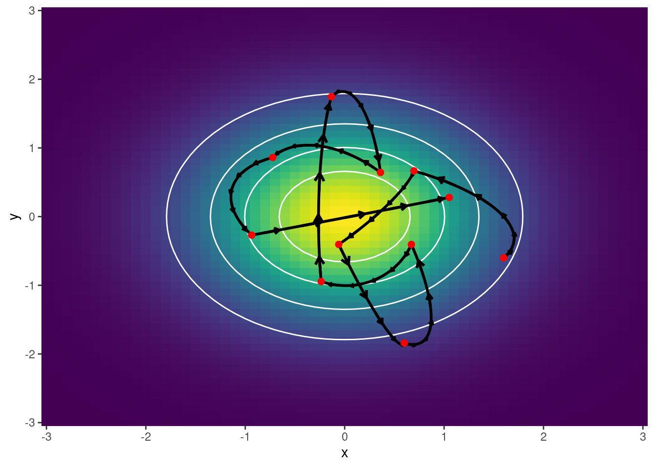
Ejemplo 2: Se obtienen muestras
neg_logp <- make_neg_logp(0)
neg_dlogp <- make_neg_dlogp(0)

initial_position <- c(1.6, -0.6)
hmc_output <- hmc(neg_logp, neg_dlogp, 1000, initial_position, 1.5, 0.01)

df_samples <- hmc_output$samples
df_leap_p <- hmc_output$leap_p
df_leap_q <- hmc_output$leap_q

df_basis <- tidyr::crossing(x1 = seq(-3.5, 3.5, 0.1), x2 = seq(-3.5, 3.5, 0.1))
plt <- df_basis |>
  dplyr::mutate(f = mvtnorm::dmvnorm(df_basis, c(0, 0), diag(2))) |>
  ggplot() +
  geom_raster(aes(x = x1, y = x2, fill = f)) +
  stat_contour(aes(x = x1, y = x2, z = f), col = "white", bins = 5) +
  viridis::scale_fill_viridis() +
  theme(
    legend.position = "none",
    plot.title = element_text(hjust = 0.5, size = 18)
  )

plt +
  geom_point(
    aes(x = x, y = y),
    size = 2,
    alpha = 0.7,
    color = "red",
    data = df_samples
  ) +
  labs(x = "x", y = "y") +
  scale_x_continuous(expand = c(0, 0)) +
  scale_y_continuous(expand = c(0, 0))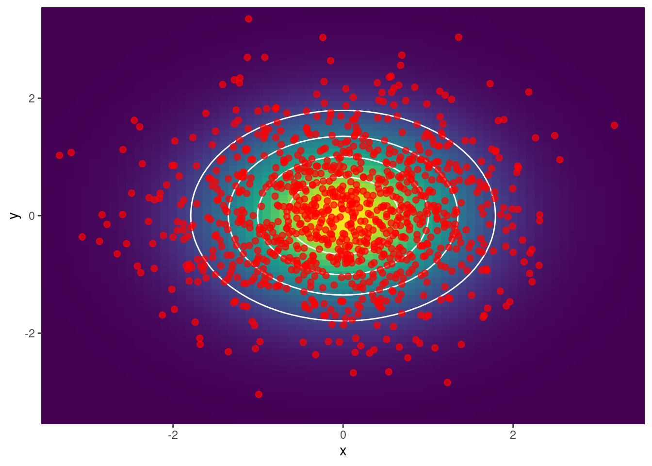
Ejemplo 3: Se obtienen muestras con \(\rho = 0.6\)
neg_logp <- make_neg_logp(0.7)
neg_dlogp <- make_neg_dlogp(0.7)

initial_position <- c(1.6, -0.6)
hmc_output <- hmc(neg_logp, neg_dlogp, 1000, initial_position, 1.5, 0.01)

df_samples <- hmc_output$samples
df_leap_p <- hmc_output$leap_p
df_leap_q <- hmc_output$leap_q

Sigma <- matrix(c(1, 0.7, 0.7, 1), ncol = 2)

df_basis <- tidyr::crossing(x1 = seq(-3.5, 3.5, 0.1), x2 = seq(-3.5, 3.5, 0.1))
plt <- df_basis |>
  dplyr::mutate(f = mvtnorm::dmvnorm(df_basis, c(0, 0), Sigma)) |>
  ggplot() +
  geom_raster(aes(x = x1, y = x2, fill = f)) +
  stat_contour(aes(x = x1, y = x2, z = f), col = "white", bins = 5) +
  viridis::scale_fill_viridis() +
  theme(
    legend.position = "none",
    plot.title = element_text(hjust = 0.5, size = 18)
  )

plt +
  geom_point(
    aes(x = x, y = y),
    size = 2,
    alpha = 0.7,
    color = "red",
    data = df_samples
  ) +
  labs(x = "x", y = "y") +
  scale_x_continuous(expand = c(0, 0)) +
  scale_y_continuous(expand = c(0, 0))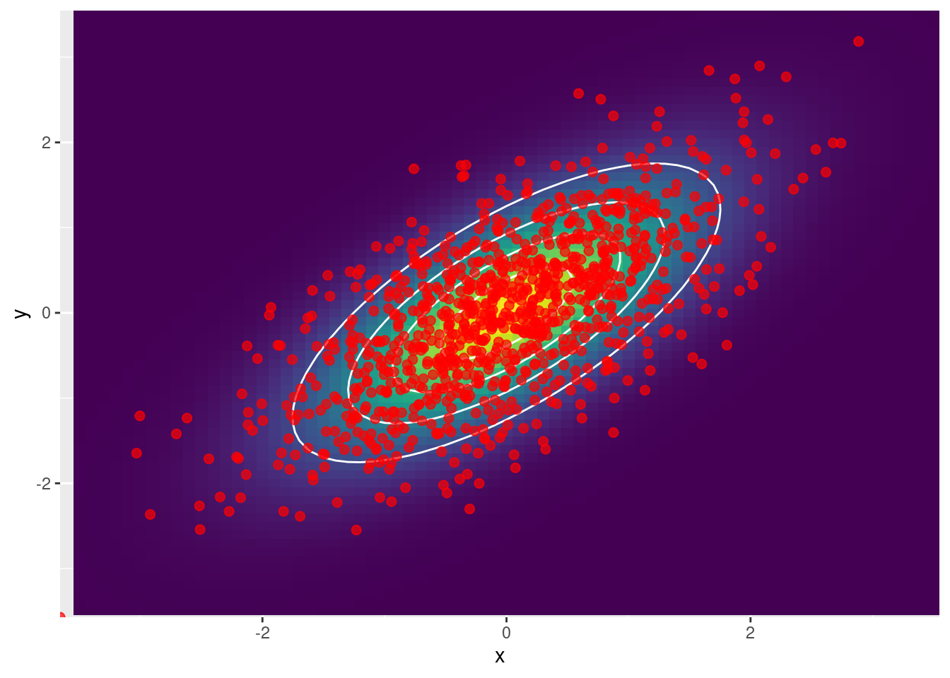
cor(df_samples$x, df_samples$y)[1] 0.6584974