# Especificar prior
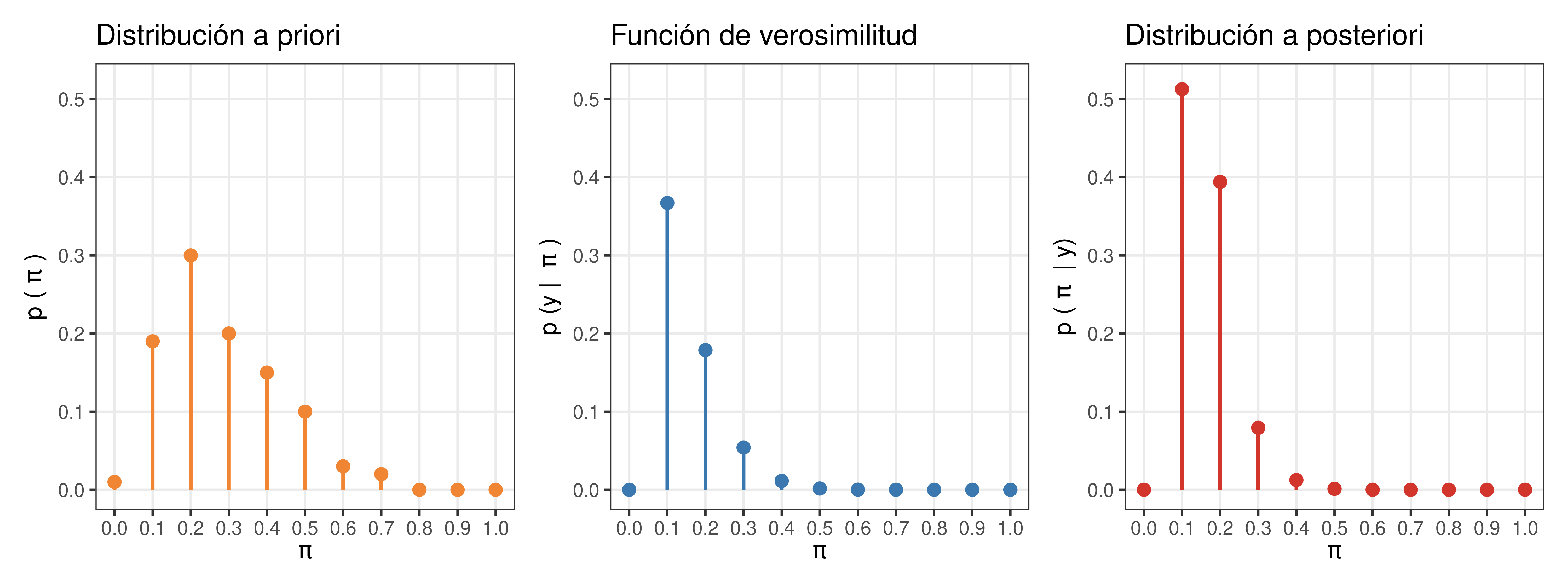
# Tenemos $1000 y los dividimos en los diferentes valores de "pi"
prior_ <- c(10, 190, 300, 200, 150, 100, 30, 20, 0, 0, 0)
prior <- prior_ / sum(prior_)

# Recolectar datos
cantidad_de_galletitas <- 13 # n
cantidad_de_melbas <- 1      # y

# Calcular verosimilitud para cada valor de "pi" en la grilla
likelihood <- dbinom(
  cantidad_de_melbas,
  cantidad_de_galletitas,
  pi_grid
)

# Obtener posterior
posterior_ <- prior * likelihood
posterior <- posterior_ / sum(posterior_) # normalización

# Graficar prior
plt_prior <- data.frame(x = pi_grid, y = prior) |>
  ggplot() +
  geom_segment(aes(x = x, xend = x, y = 0, yend = y), color = colores[1], linewidth = 0.8) +
  geom_point(aes(x = x, y = y), , color = colores[1], size = 2.4) +
  scale_y_continuous(breaks = c(0, 0.1, 0.2, 0.3, 0.4, 0.5), limits = c(0, 0.52)) +
  scale_x_continuous(breaks = pi_grid) +
  labs(
    x = expression(pi),
    y = expression(p ~ "(" ~ pi ~ ")"),
    title = "Distribución a priori"
  )

# Graficar verosimilitud
plt_likelihood <- data.frame(x = pi_grid, y = likelihood) |>
  ggplot() +
  geom_segment(aes(x = x, xend = x, y = 0, yend = y), color = colores[2], linewidth = 0.8) +
  geom_point(aes(x = x, y = y), , color = colores[2], size = 2.4) +
  scale_y_continuous(breaks = c(0, 0.1, 0.2, 0.3, 0.4, 0.5), limits = c(0, 0.52)) +
  scale_x_continuous(breaks = pi_grid) +
  labs(
    x = expression(pi),
    y = expression(p ~ "(y | " ~ pi ~ ")"),
    title = "Función de verosimilitud"
  )

# Graficar posterior
plt_posterior <- data.frame(x = pi_grid, y = posterior) |>
  ggplot() +
  geom_segment(aes(x = x, xend = x, y = 0, yend = y), color = colores[3], linewidth = 0.8) +
  geom_point(aes(x = x, y = y), , color = colores[3], size = 2.4) +
  scale_y_continuous(breaks = c(0, 0.1, 0.2, 0.3, 0.4, 0.5), limits = c(0, 0.52)) +
  scale_x_continuous(breaks = pi_grid) +
  labs(
    x = expression(pi),
    y = expression(p ~ "(" ~ pi ~ " | y)"),
    title = "Distribución a posteriori"
  )

# Concatenar graficos
plt_prior | plt_likelihood | plt_posterior