5 - Scikit-Learn para clasificación

Atribución

Este apunte es una traducción y leve adaptación de la notebook 03_classification.ipynb del repositorio ageron/handson-mlp, de Aurélien Géron. El material original se distribuye bajo la licencia Apache License 2.0. Esta versión explicita que fue traducida y adaptada para este curso.

También requiere Scikit-Learn ≥ 1.6.1:

from packaging.version import Version
import sklearn

assert Version(sklearn.__version__) >= Version("1.6.1")

MNIST

from sklearn.datasets import fetch_openml

mnist = fetch_openml("mnist_784", as_frame=False)

# código extra – es un poco largo
print(mnist.DESCR)

**Author**: Yann LeCun, Corinna Cortes, Christopher J.C. Burges  
**Source**: [MNIST Website](http://yann.lecun.com/exdb/mnist/) - Date unknown  
**Please cite**:  

The MNIST database of handwritten digits with 784 features, raw data available at: http://yann.lecun.com/exdb/mnist/. It can be split in a training set of the first 60,000 examples, and a test set of 10,000 examples  

It is a subset of a larger set available from NIST. The digits have been size-normalized and centered in a fixed-size image. It is a good database for people who want to try learning techniques and pattern recognition methods on real-world data while spending minimal efforts on preprocessing and formatting. The original black and white (bilevel) images from NIST were size normalized to fit in a 20x20 pixel box while preserving their aspect ratio. The resulting images contain grey levels as a result of the anti-aliasing technique used by the normalization algorithm. the images were centered in a 28x28 image by computing the center of mass of the pixels, and translating the image so as to position this point at the center of the 28x28 field.  

With some classification methods (particularly template-based methods, such as SVM and K-nearest neighbors), the error rate improves when the digits are centered by bounding box rather than center of mass. If you do this kind of pre-processing, you should report it in your publications. The MNIST database was constructed from NIST's NIST originally designated SD-3 as their training set and SD-1 as their test set. However, SD-3 is much cleaner and easier to recognize than SD-1. The reason for this can be found on the fact that SD-3 was collected among Census Bureau employees, while SD-1 was collected among high-school students. Drawing sensible conclusions from learning experiments requires that the result be independent of the choice of training set and test among the complete set of samples. Therefore it was necessary to build a new database by mixing NIST's datasets.  

The MNIST training set is composed of 30,000 patterns from SD-3 and 30,000 patterns from SD-1. Our test set was composed of 5,000 patterns from SD-3 and 5,000 patterns from SD-1. The 60,000 pattern training set contained examples from approximately 250 writers. We made sure that the sets of writers of the training set and test set were disjoint. SD-1 contains 58,527 digit images written by 500 different writers. In contrast to SD-3, where blocks of data from each writer appeared in sequence, the data in SD-1 is scrambled. Writer identities for SD-1 is available and we used this information to unscramble the writers. We then split SD-1 in two: characters written by the first 250 writers went into our new training set. The remaining 250 writers were placed in our test set. Thus we had two sets with nearly 30,000 examples each. The new training set was completed with enough examples from SD-3, starting at pattern # 0, to make a full set of 60,000 training patterns. Similarly, the new test set was completed with SD-3 examples starting at pattern # 35,000 to make a full set with 60,000 test patterns. Only a subset of 10,000 test images (5,000 from SD-1 and 5,000 from SD-3) is available on this site. The full 60,000 sample training set is available.

Downloaded from openml.org.

mnist.keys()  # código extra – en este notebook solo usamos data y target

dict_keys(['data', 'target', 'frame', 'categories', 'feature_names', 'target_names', 'DESCR', 'details', 'url'])

X, y = mnist.data, mnist.target
X

array([[0, 0, 0, ..., 0, 0, 0],
       [0, 0, 0, ..., 0, 0, 0],
       [0, 0, 0, ..., 0, 0, 0],
       ...,
       [0, 0, 0, ..., 0, 0, 0],
       [0, 0, 0, ..., 0, 0, 0],
       [0, 0, 0, ..., 0, 0, 0]], shape=(70000, 784))

X.shape

(70000, 784)

array(['5', '0', '4', ..., '4', '5', '6'], shape=(70000,), dtype=object)

y.shape

(70000,)

28 * 28

import matplotlib.pyplot as plt

def plot_digit(image_data):
    image = image_data.reshape(28, 28)
    plt.imshow(image, cmap="binary")
    plt.axis("off")


some_digit = X[0]
plot_digit(some_digit);

y[0]

'5'

# código extra – esta celda genera la Figura 3–2
plt.figure(figsize=(9, 9))
for idx, image_data in enumerate(X[:100]):
    plt.subplot(10, 10, idx + 1)
    plot_digit(image_data)

plt.subplots_adjust(wspace=0, hspace=0)
plt.show()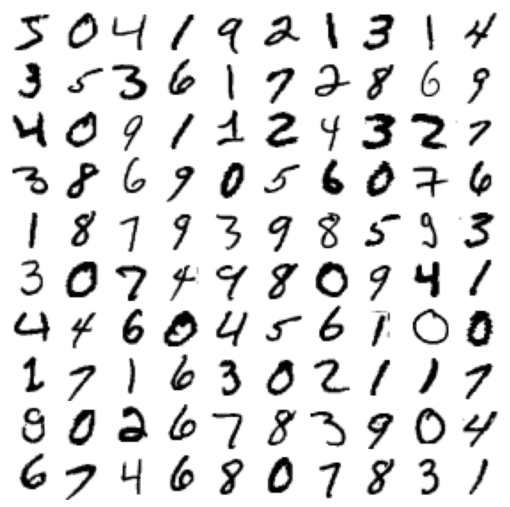

X_train, X_test, y_train, y_test = X[:60000], X[60000:], y[:60000], y[60000:]

Entrenamiento de un clasificador binario

y_train_5 = y_train == "5"  # True para todos los 5, False para todos los demás dígitos
y_test_5 = y_test == "5"

from sklearn.linear_model import SGDClassifier

sgd_clf = SGDClassifier(random_state=42)
sgd_clf.fit(X_train, y_train_5)

SGDClassifier(random_state=42)

In a Jupyter environment, please rerun this cell to show the HTML representation or trust the notebook.
On GitHub, the HTML representation is unable to render, please try loading this page with nbviewer.org.

sgd_clf.predict([some_digit])

array([ True])

Métricas de desempeño

Medición de la exactitud usando cross-validation

from sklearn.model_selection import cross_val_score

cross_val_score(sgd_clf, X_train, y_train_5, cv=3, scoring="accuracy")

array([0.95035, 0.96035, 0.9604 ])

from sklearn.model_selection import StratifiedKFold
from sklearn.base import clone

skfolds = StratifiedKFold(n_splits=3)  # agregar shuffle=True si el dataset no está mezclado
for train_index, test_index in skfolds.split(X_train, y_train_5):
    clone_clf = clone(sgd_clf)
    X_train_folds = X_train[train_index]
    y_train_folds = y_train_5[train_index]
    X_test_fold = X_train[test_index]
    y_test_fold = y_train_5[test_index]

    clone_clf.fit(X_train_folds, y_train_folds)
    y_pred = clone_clf.predict(X_test_fold)
    n_correct = sum(y_pred == y_test_fold)
    print(n_correct / len(y_pred))

0.95035
0.96035
0.9604

from sklearn.dummy import DummyClassifier

dummy_clf = DummyClassifier()
dummy_clf.fit(X_train, y_train_5)
print(any(dummy_clf.predict(X_train)))

False

cross_val_score(dummy_clf, X_train, y_train_5, cv=3, scoring="accuracy")

array([0.90965, 0.90965, 0.90965])

Matriz de confusión

from sklearn.model_selection import cross_val_predict

y_train_pred = cross_val_predict(sgd_clf, X_train, y_train_5, cv=3)

from sklearn.metrics import confusion_matrix

cm = confusion_matrix(y_train_5, y_train_pred)
cm

array([[53892,   687],
       [ 1891,  3530]])

y_train_perfect_predictions = y_train_5  # supongamos que alcanzamos la perfección
confusion_matrix(y_train_5, y_train_perfect_predictions)

array([[54579,     0],
       [    0,  5421]])

Precision y Recall

from sklearn.metrics import precision_score, recall_score

precision_score(y_train_5, y_train_pred)  # == 3530 / (687 + 3530)

0.8370879772350012

# código extra – esta celda también calcula la precision: TP / (FP + TP)
cm[1, 1] / (cm[0, 1] + cm[1, 1])

np.float64(0.8370879772350012)

recall_score(y_train_5, y_train_pred)  # == 3530 / (1891 + 3530)

0.6511713705958311

# código extra – esta celda también calcula el recall: TP / (FN + TP)
cm[1, 1] / (cm[1, 0] + cm[1, 1])

np.float64(0.6511713705958311)

from sklearn.metrics import f1_score

f1_score(y_train_5, y_train_pred)

0.7325171197343847

# código extra – esta celda también calcula el puntaje f1
cm[1, 1] / (cm[1, 1] + (cm[1, 0] + cm[0, 1]) / 2)

np.float64(0.7325171197343847)

Trade-off entre Precision y Recall

y_scores = sgd_clf.decision_function([some_digit])
y_scores

array([2164.22030239])

threshold = 0
y_some_digit_pred = y_scores > threshold

y_some_digit_pred

array([ True])

# código extra – solo muestra que y_scores > 0 produce el mismo resultado que
#              llamar a predict()
y_scores > 0

array([ True])

threshold = 3000
y_some_digit_pred = y_scores > threshold
y_some_digit_pred

array([False])

y_scores = cross_val_predict(
    sgd_clf, X_train, y_train_5, cv=3, method="decision_function"
)

from sklearn.metrics import precision_recall_curve

precisions, recalls, thresholds = precision_recall_curve(y_train_5, y_scores)

plt.figure(figsize=(8, 4))  # código extra – no hace falta, es solo formato
plt.plot(thresholds, precisions[:-1], "b--", label="Precision", linewidth=2)
plt.plot(thresholds, recalls[:-1], "g-", label="Recall", linewidth=2)
plt.vlines(threshold, 0, 1.0, "k", "dotted", label="umbral")

# código extra – esta sección solo embellece la Figura 3–5
idx = (thresholds >= threshold).argmax()  # primer índice ≥ umbral
plt.plot(thresholds[idx], precisions[idx], "bo")
plt.plot(thresholds[idx], recalls[idx], "go")
plt.axis([-50000, 50000, 0, 1])
plt.grid()
plt.xlabel("Umbral")
plt.legend(loc="center right");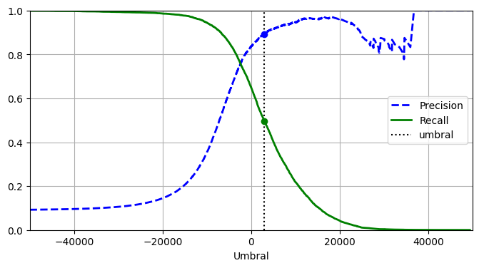

import matplotlib.patches as patches  # código extra – para la flecha curva

plt.figure(figsize=(6, 5))  # código extra – no hace falta, es solo formato

plt.plot(recalls, precisions, linewidth=2, label="Curva Precision/Recall")

# código extra – solo embellece la Figura 3–6
plt.plot([recalls[idx], recalls[idx]], [0.0, precisions[idx]], "k:")
plt.plot([0.0, recalls[idx]], [precisions[idx], precisions[idx]], "k:")
plt.plot([recalls[idx]], [precisions[idx]], "ko", label="Punto con umbral 3.000")
plt.gca().add_patch(
    patches.FancyArrowPatch(
        (0.79, 0.60),
        (0.61, 0.78),
        connectionstyle="arc3,rad=.2",
        arrowstyle="Simple, tail_width=1.5, head_width=8, head_length=10",
        color="#444444",
    )
)
plt.text(0.56, 0.62, "Umbral\nmás alto", color="#333333")
plt.xlabel("Recall")
plt.ylabel("Precision")
plt.axis([0, 1, 0, 1])
plt.grid()
plt.legend(loc="lower left");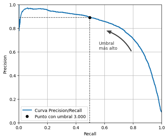

idx_for_90_precision = (precisions >= 0.90).argmax()
threshold_for_90_precision = thresholds[idx_for_90_precision]
threshold_for_90_precision

np.float64(3370.0194991439557)

y_train_pred_90 = y_scores >= threshold_for_90_precision

precision_score(y_train_5, y_train_pred_90)

0.9000345901072293

recall_at_90_precision = recall_score(y_train_5, y_train_pred_90)
recall_at_90_precision

0.4799852425751706

La curva ROC

from sklearn.metrics import roc_curve

fpr, tpr, thresholds = roc_curve(y_train_5, y_scores)

idx_for_threshold_at_90 = (thresholds <= threshold_for_90_precision).argmax()
tpr_90, fpr_90 = tpr[idx_for_threshold_at_90], fpr[idx_for_threshold_at_90]

plt.figure(figsize=(6, 5))  # código extra – no hace falta, es solo formato
plt.plot(fpr, tpr, linewidth=2, label="Curva ROC")
plt.plot([0, 1], [0, 1], "k:", label="Curva ROC de un clasificador aleatorio")
plt.plot([fpr_90], [tpr_90], "ko", label="Umbral para 90% de precision")

# código extra – solo embellece la Figura 3–7
plt.gca().add_patch(
    patches.FancyArrowPatch(
        (0.20, 0.89),
        (0.07, 0.70),
        connectionstyle="arc3,rad=.4",
        arrowstyle="Simple, tail_width=1.5, head_width=8, head_length=10",
        color="#444444",
    )
)
plt.text(0.12, 0.71, "Umbral\nmás alto", color="#333333")
plt.xlabel("Tasa de falsos positivos (Fall-Out)")
plt.ylabel("Tasa de verdaderos positivos (Recall)")
plt.grid()
plt.axis([0, 1, 0, 1])
plt.legend(loc="lower right", fontsize=13)

plt.show()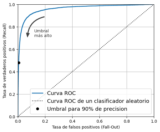

from sklearn.metrics import roc_auc_score

roc_auc_score(y_train_5, y_scores)

0.9604938554008616

Advertencia: la siguiente celda puede tardar unos minutos en ejecutarse.

from sklearn.ensemble import RandomForestClassifier

forest_clf = RandomForestClassifier(random_state=42)

y_probas_forest = cross_val_predict(
    forest_clf, X_train, y_train_5, cv=3, method="predict_proba"
)

y_probas_forest[:2]

array([[0.11, 0.89],
       [0.99, 0.01]])

Estas son probabilidades estimadas. Entre las imágenes que el modelo clasificó como positivas con una probabilidad entre 50% y 60%, en realidad hay alrededor de un 94% de imágenes positivas:

# No está en el código
idx_50_to_60 = (y_probas_forest[:, 1] > 0.50) & (y_probas_forest[:, 1] < 0.60)
print(f"{(y_train_5[idx_50_to_60]).sum() / idx_50_to_60.sum():.1%}")

94.0%

y_scores_forest = y_probas_forest[:, 1]
precisions_forest, recalls_forest, thresholds_forest = precision_recall_curve(
    y_train_5, y_scores_forest
)

plt.figure(figsize=(6, 5))  # código extra – no hace falta, es solo formato

plt.plot(recalls_forest, precisions_forest, "b-", linewidth=2, label="Random Forest")
plt.plot(recalls, precisions, "--", linewidth=2, label="SGD")

# código extra – solo embellece la Figura 3–8
plt.xlabel("Recall")
plt.ylabel("Precision")
plt.axis([0, 1, 0, 1])
plt.grid()
plt.legend(loc="lower left");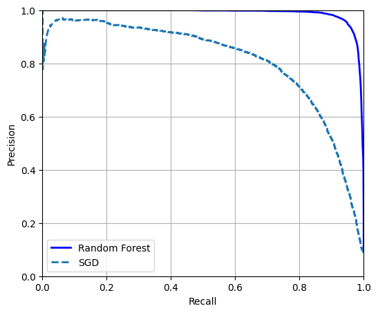

Podríamos usar cross_val_predict(forest_clf, X_train, y_train_5, cv=3) para calcular y_train_pred_forest, pero como ya tenemos las probabilidades estimadas, podemos simplemente usar el umbral predeterminado de 50% de probabilidad para obtener las mismas predicciones mucho más rápido:

y_train_pred_forest = y_probas_forest[:, 1] >= 0.5  # proba positiva ≥ 50%
f1_score(y_train_5, y_train_pred_forest)

0.9274509803921569

roc_auc_score(y_train_5, y_scores_forest)

0.9983436731328145

precision_score(y_train_5, y_train_pred_forest)

0.9897468089558485

recall_score(y_train_5, y_train_pred_forest)

0.8725327430363402

Clasificación multiclase

Los SVM no escalan bien con datasets grandes, así que entrenemos solo con las primeras 2.000 instancias; de lo contrario, esta sección tardará muchísimo en ejecutarse:

from sklearn.svm import SVC

svm_clf = SVC(random_state=42)
svm_clf.fit(X_train[:2000], y_train[:2000])  # y_train, no y_train_5

SVC(random_state=42)

svm_clf.predict([some_digit])

array(['5'], dtype=object)

some_digit_scores = svm_clf.decision_function([some_digit])
some_digit_scores.round(2)

array([[ 3.79,  0.73,  6.06,  8.3 , -0.29,  9.3 ,  1.75,  2.77,  7.21,
         4.82]])

class_id = some_digit_scores.argmax()
class_id

np.int64(5)

svm_clf.classes_

array(['0', '1', '2', '3', '4', '5', '6', '7', '8', '9'], dtype=object)

svm_clf.classes_[class_id]

'5'

Si querés que decision_function() devuelva los 45 puntajes, podés establecer el hiperparámetro decision_function_shape en "ovo". El valor predeterminado es "ovr", pero no dejes que eso te confunda: SVC siempre usa OvO para entrenar. Este hiperparámetro solo afecta si los 45 puntajes se agregan o no:

# código extra – muestra cómo obtener los 45 puntajes OvO si hace falta
svm_clf.decision_function_shape = "ovo"
some_digit_scores_ovo = svm_clf.decision_function([some_digit])
some_digit_scores_ovo.round(2)

array([[ 0.11, -0.21, -0.97,  0.51, -1.01,  0.19,  0.09, -0.31, -0.04,
        -0.45, -1.28,  0.25, -1.01, -0.13, -0.32, -0.9 , -0.36, -0.93,
         0.79, -1.  ,  0.45,  0.24, -0.24,  0.25,  1.54, -0.77,  1.11,
         1.13,  1.04,  1.2 , -1.42, -0.53, -0.45, -0.99, -0.95,  1.21,
         1.  ,  1.  ,  1.08, -0.02, -0.67, -0.14, -0.3 , -0.13,  0.25]])

from sklearn.multiclass import OneVsRestClassifier

ovr_clf = OneVsRestClassifier(SVC(random_state=42))
ovr_clf.fit(X_train[:2000], y_train[:2000])

OneVsRestClassifier(estimator=SVC(random_state=42))

ovr_clf.predict([some_digit])

array(['5'], dtype='<U1')

len(ovr_clf.estimators_)

sgd_clf = SGDClassifier(random_state=42)
sgd_clf.fit(X_train, y_train)
sgd_clf.predict([some_digit])

array(['3'], dtype='<U1')

sgd_clf.decision_function([some_digit]).round()

array([[-31893., -19048.,  -9531.,   1824., -22320.,  -1386., -26189.,
        -16148.,  -4604., -12051.]])

Advertencia: las dos celdas siguientes pueden tardar unos minutos cada una en ejecutarse:

cross_val_score(sgd_clf, X_train, y_train, cv=3, scoring="accuracy")

array([0.87745, 0.85835, 0.8698 ])

from sklearn.preprocessing import StandardScaler

scaler = StandardScaler()
X_train_scaled = scaler.fit_transform(X_train.astype("float64"))
cross_val_score(sgd_clf, X_train_scaled, y_train, cv=3, scoring="accuracy")

/home/tomas/miniconda3/lib/python3.13/site-packages/sklearn/linear_model/_stochastic_gradient.py:733: ConvergenceWarning: Maximum number of iteration reached before convergence. Consider increasing max_iter to improve the fit.
  warnings.warn(
/home/tomas/miniconda3/lib/python3.13/site-packages/sklearn/linear_model/_stochastic_gradient.py:733: ConvergenceWarning: Maximum number of iteration reached before convergence. Consider increasing max_iter to improve the fit.
  warnings.warn(
/home/tomas/miniconda3/lib/python3.13/site-packages/sklearn/linear_model/_stochastic_gradient.py:733: ConvergenceWarning: Maximum number of iteration reached before convergence. Consider increasing max_iter to improve the fit.
  warnings.warn(

array([0.89835, 0.8902 , 0.90095])

Análisis de errores

Advertencia: la siguiente celda tardará unos minutos en ejecutarse:

from sklearn.metrics import ConfusionMatrixDisplay

y_train_pred = cross_val_predict(sgd_clf, X_train_scaled, y_train, cv=3)
ConfusionMatrixDisplay.from_predictions(y_train, y_train_pred);

/home/tomas/miniconda3/lib/python3.13/site-packages/sklearn/linear_model/_stochastic_gradient.py:733: ConvergenceWarning: Maximum number of iteration reached before convergence. Consider increasing max_iter to improve the fit.
  warnings.warn(
/home/tomas/miniconda3/lib/python3.13/site-packages/sklearn/linear_model/_stochastic_gradient.py:733: ConvergenceWarning: Maximum number of iteration reached before convergence. Consider increasing max_iter to improve the fit.
  warnings.warn(
/home/tomas/miniconda3/lib/python3.13/site-packages/sklearn/linear_model/_stochastic_gradient.py:733: ConvergenceWarning: Maximum number of iteration reached before convergence. Consider increasing max_iter to improve the fit.
  warnings.warn(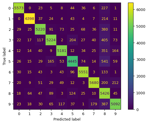

ConfusionMatrixDisplay.from_predictions(y_train, y_train_pred, normalize="true", values_format=".0%");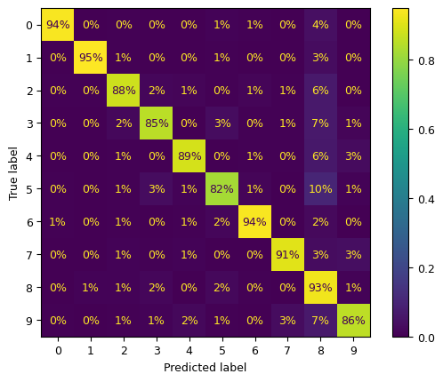

sample_weight = y_train_pred != y_train
ConfusionMatrixDisplay.from_predictions(
    y_train,
    y_train_pred,
    sample_weight=sample_weight,
    normalize="true",
    values_format=".0%",
);

Pongamos todos los gráficos en un par de figuras para el libro:

fig, axs = plt.subplots(nrows=1, ncols=2, figsize=(12, 5))
ConfusionMatrixDisplay.from_predictions(y_train, y_train_pred, ax=axs[0])
ConfusionMatrixDisplay.from_predictions(
    y_train, y_train_pred, ax=axs[1], normalize="true", values_format=".0%"
)
axs[0].set_title("Matriz de confusión")
axs[1].set_title("MC normalizada por fila");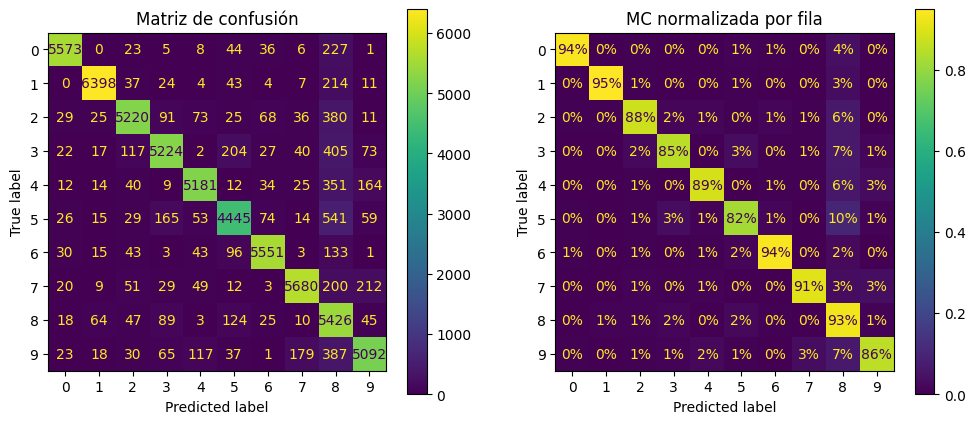

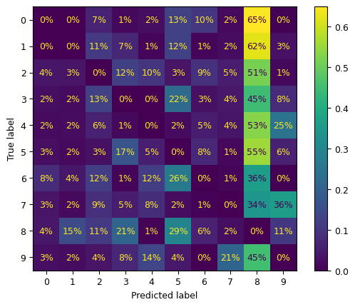
# código extra – esta celda genera la Figura 3–10
fig, axs = plt.subplots(nrows=1, ncols=2, figsize=(15, 5))
ConfusionMatrixDisplay.from_predictions(
    y_train,
    y_train_pred,
    ax=axs[0],
    sample_weight=sample_weight,
    normalize="true",
    values_format=".0%",
)
ConfusionMatrixDisplay.from_predictions(
    y_train,
    y_train_pred,
    ax=axs[1],
    sample_weight=sample_weight,
    normalize="pred",
    values_format=".0%",
)
axs[0].set_title("Errores normalizados por fila")
axs[1].set_title("Errores normalizados por columna");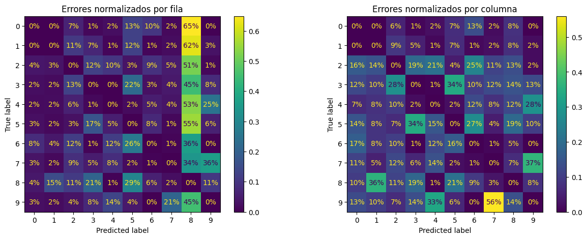

cl_a, cl_b = "3", "5"
X_aa = X_train[(y_train == cl_a) & (y_train_pred == cl_a)]
X_ab = X_train[(y_train == cl_a) & (y_train_pred == cl_b)]
X_ba = X_train[(y_train == cl_b) & (y_train_pred == cl_a)]
X_bb = X_train[(y_train == cl_b) & (y_train_pred == cl_b)]

# código extra – esta celda genera la Figura 3–11
size = 5
pad = 0.2
plt.figure(figsize=(size, size))
for images, (label_col, label_row) in [
    (X_ba, (0, 0)),
    (X_bb, (1, 0)),
    (X_aa, (0, 1)),
    (X_ab, (1, 1)),
]:
    for idx, image_data in enumerate(images[: size * size]):
        x = idx % size + label_col * (size + pad)
        y = idx // size + label_row * (size + pad)
        plt.imshow(
            image_data.reshape(28, 28), cmap="binary", extent=(x, x + 1, y, y + 1)
        )
plt.xticks([size / 2, size + pad + size / 2], [str(cl_a), str(cl_b)])
plt.yticks([size / 2, size + pad + size / 2], [str(cl_b), str(cl_a)])
plt.plot([size + pad / 2, size + pad / 2], [0, 2 * size + pad], "k:")
plt.plot([0, 2 * size + pad], [size + pad / 2, size + pad / 2], "k:")
plt.axis([0, 2 * size + pad, 0, 2 * size + pad])
plt.xlabel("Etiqueta predicha")
plt.ylabel("Etiqueta real");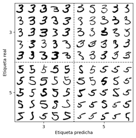

Nota: hay varias otras formas de programar un gráfico como este, pero es un poco difícil lograr que las etiquetas de los ejes queden bien: * usando GridSpecs anidados * fusionando todos los dígitos de cada bloque en una sola imagen (y luego usando subplots de 2×2). Por ejemplo: python X_aa[:25].reshape(5, 5, 28, 28).transpose(0, 2, 1, 3).reshape(5 * 28, 5 * 28) * usando subfigures (desde Matplotlib 3.4)

Clasificación multilabel

import numpy as np
from sklearn.neighbors import KNeighborsClassifier

y_train_large = y_train >= "7"
y_train_odd = y_train.astype("int8") % 2 == 1
y_multilabel = np.c_[y_train_large, y_train_odd]

knn_clf = KNeighborsClassifier()
knn_clf.fit(X_train, y_multilabel)

KNeighborsClassifier()

knn_clf.predict([some_digit])

array([[False,  True]])

Advertencia: la siguiente celda puede tardar unos minutos en ejecutarse:

y_train_knn_pred = cross_val_predict(knn_clf, X_train, y_multilabel, cv=3)
f1_score(y_multilabel, y_train_knn_pred, average="macro")

0.9764102655606048

# código extra – muestra que obtenemos una mejora de desempeño despreciable al
#              establecer average="weighted" porque las clases ya están bastante
#              bien balanceadas.
f1_score(y_multilabel, y_train_knn_pred, average="weighted")

0.9778357403921755

from sklearn.multioutput import ClassifierChain

chain_clf = ClassifierChain(SVC(), cv=3, random_state=42)
chain_clf.fit(X_train[:2000], y_multilabel[:2000])

ClassifierChain(cv=3, estimator=SVC(), random_state=42)

chain_clf.predict([some_digit])

array([[0., 1.]])

Clasificación multioutput

rng = np.random.default_rng(seed=42)  # para hacer este ejemplo de código reproducible
noise_train = rng.integers(0, 100, (len(X_train), 784))
X_train_mod = X_train + noise_train
noise_test = rng.integers(0, 100, (len(X_test), 784))
X_test_mod = X_test + noise_test
y_train_mod = X_train
y_test_mod = X_test

# código extra – esta celda genera la Figura 3–12
plt.subplot(121)
plot_digit(X_test_mod[0])
plt.subplot(122)
plot_digit(y_test_mod[0]);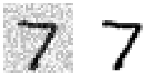

knn_clf = KNeighborsClassifier()
knn_clf.fit(X_train_mod, y_train_mod)
clean_digit = knn_clf.predict([X_test_mod[0]])
plot_digit(clean_digit);

	loss loss: {'hinge', 'log_loss', 'modified_huber', 'squared_hinge', 'perceptron', 'squared_error', 'huber', 'epsilon_insensitive', 'squared_epsilon_insensitive'}, default='hinge' The loss function to be used. - 'hinge' gives a linear SVM. - 'log_loss' gives logistic regression, a probabilistic classifier. - 'modified_huber' is another smooth loss that brings tolerance to outliers as well as probability estimates. - 'squared_hinge' is like hinge but is quadratically penalized. - 'perceptron' is the linear loss used by the perceptron algorithm. - The other losses, 'squared_error', 'huber', 'epsilon_insensitive' and 'squared_epsilon_insensitive' are designed for regression but can be useful in classification as well; see :class:`~sklearn.linear_model.SGDRegressor` for a description. More details about the losses formulas can be found in the :ref:`User Guide ` and you can find a visualisation of the loss functions in :ref:`sphx_glr_auto_examples_linear_model_plot_sgd_loss_functions.py`.	'hinge'
	penalty penalty: {'l2', 'l1', 'elasticnet', None}, default='l2' The penalty (aka regularization term) to be used. Defaults to 'l2' which is the standard regularizer for linear SVM models. 'l1' and 'elasticnet' might bring sparsity to the model (feature selection) not achievable with 'l2'. No penalty is added when set to `None`. You can see a visualisation of the penalties in :ref:`sphx_glr_auto_examples_linear_model_plot_sgd_penalties.py`.	'l2'
	alpha alpha: float, default=0.0001 Constant that multiplies the regularization term. The higher the value, the stronger the regularization. Also used to compute the learning rate when `learning_rate` is set to 'optimal'. Values must be in the range `[0.0, inf)`.	0.0001
	l1_ratio l1_ratio: float, default=0.15 The Elastic Net mixing parameter, with 0 <= l1_ratio <= 1. l1_ratio=0 corresponds to L2 penalty, l1_ratio=1 to L1. Only used if `penalty` is 'elasticnet'. Values must be in the range `[0.0, 1.0]` or can be `None` if `penalty` is not `elasticnet`. .. versionchanged:: 1.7 `l1_ratio` can be `None` when `penalty` is not "elasticnet".	0.15
	fit_intercept fit_intercept: bool, default=True Whether the intercept should be estimated or not. If False, the data is assumed to be already centered.	True
	max_iter max_iter: int, default=1000 The maximum number of passes over the training data (aka epochs). It only impacts the behavior in the ``fit`` method, and not the :meth:`partial_fit` method. Values must be in the range `[1, inf)`. .. versionadded:: 0.19	1000
	tol tol: float or None, default=1e-3 The stopping criterion. If it is not None, training will stop when (loss > best_loss - tol) for ``n_iter_no_change`` consecutive epochs. Convergence is checked against the training loss or the validation loss depending on the `early_stopping` parameter. Values must be in the range `[0.0, inf)`. .. versionadded:: 0.19	0.001
	shuffle shuffle: bool, default=True Whether or not the training data should be shuffled after each epoch.	True
	verbose verbose: int, default=0 The verbosity level. Values must be in the range `[0, inf)`.	0
	epsilon epsilon: float, default=0.1 Epsilon in the epsilon-insensitive loss functions; only if `loss` is 'huber', 'epsilon_insensitive', or 'squared_epsilon_insensitive'. For 'huber', determines the threshold at which it becomes less important to get the prediction exactly right. For epsilon-insensitive, any differences between the current prediction and the correct label are ignored if they are less than this threshold. Values must be in the range `[0.0, inf)`.	0.1
	n_jobs n_jobs: int, default=None The number of CPUs to use to do the OVA (One Versus All, for multi-class problems) computation. ``None`` means 1 unless in a :obj:`joblib.parallel_backend` context. ``-1`` means using all processors. See :term:`Glossary ` for more details.	None
	random_state random_state: int, RandomState instance, default=None Used for shuffling the data, when ``shuffle`` is set to ``True``. Pass an int for reproducible output across multiple function calls. See :term:`Glossary `. Integer values must be in the range `[0, 2**32 - 1]`.	42
	learning_rate learning_rate: str, default='optimal' The learning rate schedule: - 'constant': `eta = eta0` - 'optimal': `eta = 1.0 / (alpha * (t + t0))` where `t0` is chosen by a heuristic proposed by Leon Bottou. - 'invscaling': `eta = eta0 / pow(t, power_t)` - 'adaptive': `eta = eta0`, as long as the training keeps decreasing. Each time n_iter_no_change consecutive epochs fail to decrease the training loss by tol or fail to increase validation score by tol if `early_stopping` is `True`, the current learning rate is divided by 5. - 'pa1': passive-aggressive algorithm 1, see [1]_. Only with `loss='hinge'`. Update is `w += eta y x` with `eta = min(eta0, loss/\|\|x\|\|2)`. - 'pa2': passive-aggressive algorithm 2, see [1]_. Only with `loss='hinge'`. Update is `w += eta y x` with `eta = hinge_loss / (\|\|x\|\|2 + 1/(2 eta0))`. .. versionadded:: 0.20 Added 'adaptive' option. .. versionadded:: 1.8 Added options 'pa1' and 'pa2'	'optimal'
	eta0 eta0: float, default=0.01 The initial learning rate for the 'constant', 'invscaling' or 'adaptive' schedules. The default value is 0.01, but note that eta0 is not used by the default learning rate 'optimal'. Values must be in the range `(0.0, inf)`. For PA-1 (`learning_rate=pa1`) and PA-II (`pa2`), it specifies the aggressiveness parameter for the passive-agressive algorithm, see [1] where it is called C: - For PA-I it is the maximum step size. - For PA-II it regularizes the step size (the smaller `eta0` the more it regularizes). As a general rule-of-thumb for PA, `eta0` should be small when the data is noisy.	0.01
	power_t power_t: float, default=0.5 The exponent for inverse scaling learning rate. Values must be in the range `[0.0, inf)`. .. deprecated:: 1.8 Negative values for `power_t` are deprecated in version 1.8 and will raise an error in 1.10. Use values in the range [0.0, inf) instead.	0.5
	early_stopping early_stopping: bool, default=False Whether to use early stopping to terminate training when validation score is not improving. If set to `True`, it will automatically set aside a stratified fraction of training data as validation and terminate training when validation score returned by the `score` method is not improving by at least tol for n_iter_no_change consecutive epochs. See :ref:`sphx_glr_auto_examples_linear_model_plot_sgd_early_stopping.py` for an example of the effects of early stopping. .. versionadded:: 0.20 Added 'early_stopping' option	False
	validation_fraction validation_fraction: float, default=0.1 The proportion of training data to set aside as validation set for early stopping. Must be between 0 and 1. Only used if `early_stopping` is True. Values must be in the range `(0.0, 1.0)`. .. versionadded:: 0.20 Added 'validation_fraction' option	0.1
	n_iter_no_change n_iter_no_change: int, default=5 Number of iterations with no improvement to wait before stopping fitting. Convergence is checked against the training loss or the validation loss depending on the `early_stopping` parameter. Integer values must be in the range `[1, max_iter)`. .. versionadded:: 0.20 Added 'n_iter_no_change' option	5
	class_weight class_weight: dict, {class_label: weight} or "balanced", default=None Preset for the class_weight fit parameter. Weights associated with classes. If not given, all classes are supposed to have weight one. The "balanced" mode uses the values of y to automatically adjust weights inversely proportional to class frequencies in the input data as ``n_samples / (n_classes * np.bincount(y))``.	None
	warm_start warm_start: bool, default=False When set to True, reuse the solution of the previous call to fit as initialization, otherwise, just erase the previous solution. See :term:`the Glossary `. Repeatedly calling fit or partial_fit when warm_start is True can result in a different solution than when calling fit a single time because of the way the data is shuffled. If a dynamic learning rate is used, the learning rate is adapted depending on the number of samples already seen. Calling ``fit`` resets this counter, while ``partial_fit`` will result in increasing the existing counter.	False
	average average: bool or int, default=False When set to `True`, computes the averaged SGD weights across all updates and stores the result in the ``coef_`` attribute. If set to an int greater than 1, averaging will begin once the total number of samples seen reaches `average`. So ``average=10`` will begin averaging after seeing 10 samples. Integer values must be in the range `[1, n_samples]`.	False

	C C: float, default=1.0 Regularization parameter. The strength of the regularization is inversely proportional to C. Must be strictly positive. The penalty is a squared l2 penalty. For an intuitive visualization of the effects of scaling the regularization parameter C, see :ref:`sphx_glr_auto_examples_svm_plot_svm_scale_c.py`.	1.0
	kernel kernel: {'linear', 'poly', 'rbf', 'sigmoid', 'precomputed'} or callable, default='rbf' Specifies the kernel type to be used in the algorithm. If none is given, 'rbf' will be used. If a callable is given it is used to pre-compute the kernel matrix from data matrices; that matrix should be an array of shape ``(n_samples, n_samples)``. For an intuitive visualization of different kernel types see :ref:`sphx_glr_auto_examples_svm_plot_svm_kernels.py`.	'rbf'
	degree degree: int, default=3 Degree of the polynomial kernel function ('poly'). Must be non-negative. Ignored by all other kernels.	3
	gamma gamma: {'scale', 'auto'} or float, default='scale' Kernel coefficient for 'rbf', 'poly' and 'sigmoid'. - if ``gamma='scale'`` (default) is passed then it uses 1 / (n_features * X.var()) as value of gamma, - if 'auto', uses 1 / n_features - if float, must be non-negative. .. versionchanged:: 0.22 The default value of ``gamma`` changed from 'auto' to 'scale'.	'scale'
	coef0 coef0: float, default=0.0 Independent term in kernel function. It is only significant in 'poly' and 'sigmoid'.	0.0
	shrinking shrinking: bool, default=True Whether to use the shrinking heuristic. See the :ref:`User Guide `.	True
	probability probability: bool, default=False Whether to enable probability estimates. This must be enabled prior to calling `fit`, will slow down that method as it internally uses 5-fold cross-validation, and `predict_proba` may be inconsistent with `predict`. Read more in the :ref:`User Guide `.	False
	tol tol: float, default=1e-3 Tolerance for stopping criterion.	0.001
	cache_size cache_size: float, default=200 Specify the size of the kernel cache (in MB).	200
	class_weight class_weight: dict or 'balanced', default=None Set the parameter C of class i to class_weight[i]C for SVC. If not given, all classes are supposed to have weight one. The "balanced" mode uses the values of y to automatically adjust weights inversely proportional to class frequencies in the input data as ``n_samples / (n_classes np.bincount(y))``.	None
	verbose verbose: bool, default=False Enable verbose output. Note that this setting takes advantage of a per-process runtime setting in libsvm that, if enabled, may not work properly in a multithreaded context.	False
	max_iter max_iter: int, default=-1 Hard limit on iterations within solver, or -1 for no limit.	-1
	decision_function_shape decision_function_shape: {'ovo', 'ovr'}, default='ovr' Whether to return a one-vs-rest ('ovr') decision function of shape (n_samples, n_classes) as all other classifiers, or the original one-vs-one ('ovo') decision function of libsvm which has shape (n_samples, n_classes * (n_classes - 1) / 2). However, note that internally, one-vs-one ('ovo') is always used as a multi-class strategy to train models; an ovr matrix is only constructed from the ovo matrix. The parameter is ignored for binary classification. .. versionchanged:: 0.19 decision_function_shape is 'ovr' by default. .. versionadded:: 0.17 decision_function_shape='ovr' is recommended. .. versionchanged:: 0.17 Deprecated decision_function_shape='ovo' and None.	'ovr'
	break_ties break_ties: bool, default=False If true, ``decision_function_shape='ovr'``, and number of classes > 2, :term:`predict` will break ties according to the confidence values of :term:`decision_function`; otherwise the first class among the tied classes is returned. Please note that breaking ties comes at a relatively high computational cost compared to a simple predict. See :ref:`sphx_glr_auto_examples_svm_plot_svm_tie_breaking.py` for an example of its usage with ``decision_function_shape='ovr'``. .. versionadded:: 0.22	False
	random_state random_state: int, RandomState instance or None, default=None Controls the pseudo random number generation for shuffling the data for probability estimates. Ignored when `probability` is False. Pass an int for reproducible output across multiple function calls. See :term:`Glossary `.	42

	estimator estimator: estimator object A regressor or a classifier that implements :term:`fit`. When a classifier is passed, :term:`decision_function` will be used in priority and it will fallback to :term:`predict_proba` if it is not available. When a regressor is passed, :term:`predict` is used.	SVC(random_state=42)
	n_jobs n_jobs: int, default=None The number of jobs to use for the computation: the `n_classes` one-vs-rest problems are computed in parallel. ``None`` means 1 unless in a :obj:`joblib.parallel_backend` context. ``-1`` means using all processors. See :term:`Glossary ` for more details. .. versionchanged:: 0.20 `n_jobs` default changed from 1 to None	None
	verbose verbose: int, default=0 The verbosity level, if non zero, progress messages are printed. Below 50, the output is sent to stderr. Otherwise, the output is sent to stdout. The frequency of the messages increases with the verbosity level, reporting all iterations at 10. See :class:`joblib.Parallel` for more details. .. versionadded:: 1.1	0

	C C: float, default=1.0 Regularization parameter. The strength of the regularization is inversely proportional to C. Must be strictly positive. The penalty is a squared l2 penalty. For an intuitive visualization of the effects of scaling the regularization parameter C, see :ref:`sphx_glr_auto_examples_svm_plot_svm_scale_c.py`.	1.0
	kernel kernel: {'linear', 'poly', 'rbf', 'sigmoid', 'precomputed'} or callable, default='rbf' Specifies the kernel type to be used in the algorithm. If none is given, 'rbf' will be used. If a callable is given it is used to pre-compute the kernel matrix from data matrices; that matrix should be an array of shape ``(n_samples, n_samples)``. For an intuitive visualization of different kernel types see :ref:`sphx_glr_auto_examples_svm_plot_svm_kernels.py`.	'rbf'
	degree degree: int, default=3 Degree of the polynomial kernel function ('poly'). Must be non-negative. Ignored by all other kernels.	3
	gamma gamma: {'scale', 'auto'} or float, default='scale' Kernel coefficient for 'rbf', 'poly' and 'sigmoid'. - if ``gamma='scale'`` (default) is passed then it uses 1 / (n_features * X.var()) as value of gamma, - if 'auto', uses 1 / n_features - if float, must be non-negative. .. versionchanged:: 0.22 The default value of ``gamma`` changed from 'auto' to 'scale'.	'scale'
	coef0 coef0: float, default=0.0 Independent term in kernel function. It is only significant in 'poly' and 'sigmoid'.	0.0
	shrinking shrinking: bool, default=True Whether to use the shrinking heuristic. See the :ref:`User Guide `.	True
	probability probability: bool, default=False Whether to enable probability estimates. This must be enabled prior to calling `fit`, will slow down that method as it internally uses 5-fold cross-validation, and `predict_proba` may be inconsistent with `predict`. Read more in the :ref:`User Guide `.	False
	tol tol: float, default=1e-3 Tolerance for stopping criterion.	0.001
	cache_size cache_size: float, default=200 Specify the size of the kernel cache (in MB).	200
	class_weight class_weight: dict or 'balanced', default=None Set the parameter C of class i to class_weight[i]C for SVC. If not given, all classes are supposed to have weight one. The "balanced" mode uses the values of y to automatically adjust weights inversely proportional to class frequencies in the input data as ``n_samples / (n_classes np.bincount(y))``.	None
	verbose verbose: bool, default=False Enable verbose output. Note that this setting takes advantage of a per-process runtime setting in libsvm that, if enabled, may not work properly in a multithreaded context.	False
	max_iter max_iter: int, default=-1 Hard limit on iterations within solver, or -1 for no limit.	-1
	decision_function_shape decision_function_shape: {'ovo', 'ovr'}, default='ovr' Whether to return a one-vs-rest ('ovr') decision function of shape (n_samples, n_classes) as all other classifiers, or the original one-vs-one ('ovo') decision function of libsvm which has shape (n_samples, n_classes * (n_classes - 1) / 2). However, note that internally, one-vs-one ('ovo') is always used as a multi-class strategy to train models; an ovr matrix is only constructed from the ovo matrix. The parameter is ignored for binary classification. .. versionchanged:: 0.19 decision_function_shape is 'ovr' by default. .. versionadded:: 0.17 decision_function_shape='ovr' is recommended. .. versionchanged:: 0.17 Deprecated decision_function_shape='ovo' and None.	'ovr'
	break_ties break_ties: bool, default=False If true, ``decision_function_shape='ovr'``, and number of classes > 2, :term:`predict` will break ties according to the confidence values of :term:`decision_function`; otherwise the first class among the tied classes is returned. Please note that breaking ties comes at a relatively high computational cost compared to a simple predict. See :ref:`sphx_glr_auto_examples_svm_plot_svm_tie_breaking.py` for an example of its usage with ``decision_function_shape='ovr'``. .. versionadded:: 0.22	False
	random_state random_state: int, RandomState instance or None, default=None Controls the pseudo random number generation for shuffling the data for probability estimates. Ignored when `probability` is False. Pass an int for reproducible output across multiple function calls. See :term:`Glossary `.	42

	n_neighbors n_neighbors: int, default=5 Number of neighbors to use by default for :meth:`kneighbors` queries.	5
	weights weights: {'uniform', 'distance'}, callable or None, default='uniform' Weight function used in prediction. Possible values: - 'uniform' : uniform weights. All points in each neighborhood are weighted equally. - 'distance' : weight points by the inverse of their distance. in this case, closer neighbors of a query point will have a greater influence than neighbors which are further away. - [callable] : a user-defined function which accepts an array of distances, and returns an array of the same shape containing the weights. Refer to the example entitled :ref:`sphx_glr_auto_examples_neighbors_plot_classification.py` showing the impact of the `weights` parameter on the decision boundary.	'uniform'
	algorithm algorithm: {'auto', 'ball_tree', 'kd_tree', 'brute'}, default='auto' Algorithm used to compute the nearest neighbors: - 'ball_tree' will use :class:`BallTree` - 'kd_tree' will use :class:`KDTree` - 'brute' will use a brute-force search. - 'auto' will attempt to decide the most appropriate algorithm based on the values passed to :meth:`fit` method. Note: fitting on sparse input will override the setting of this parameter, using brute force.	'auto'
	leaf_size leaf_size: int, default=30 Leaf size passed to BallTree or KDTree. This can affect the speed of the construction and query, as well as the memory required to store the tree. The optimal value depends on the nature of the problem.	30
	p p: float, default=2 Power parameter for the Minkowski metric. When p = 1, this is equivalent to using manhattan_distance (l1), and euclidean_distance (l2) for p = 2. For arbitrary p, minkowski_distance (l_p) is used. This parameter is expected to be positive.	2
	metric metric: str or callable, default='minkowski' Metric to use for distance computation. Default is "minkowski", which results in the standard Euclidean distance when p = 2. See the documentation of `scipy.spatial.distance < docs.scipy.org doc scipy reference spatial.distance.html>`_ and the metrics listed in :class:`~sklearn.metrics.pairwise.distance_metrics` for valid metric values. If metric is "precomputed", X is assumed to be a distance matrix and must be square during fit. X may be a :term:`sparse graph`, in which case only "nonzero" elements may be considered neighbors. If metric is a callable function, it takes two arrays representing 1D vectors as inputs and must return one value indicating the distance between those vectors. This works for Scipy's metrics, but is less efficient than passing the metric name as a string.	'minkowski'
	metric_params metric_params: dict, default=None Additional keyword arguments for the metric function.	None
	n_jobs n_jobs: int, default=None The number of parallel jobs to run for neighbors search. ``None`` means 1 unless in a :obj:`joblib.parallel_backend` context. ``-1`` means using all processors. See :term:`Glossary ` for more details. Doesn't affect :meth:`fit` method.	None