4 - Proyecto de ML

Atribución

Este apunte es una traducción y leve adaptación de la notebook 02_end_to_end_machine_learning_project.ipynb del repositorio ageron/handson-mlp, de Aurélien Géron. El material original se distribuye bajo la licencia Apache License 2.0. Esta versión explicita que fue traducida y adaptada para este curso.

Requiere Scikit-Learn ≥ 1.6.1:

from packaging.version import Version
import sklearn

assert Version(sklearn.__version__) >= Version("1.6.1")

Obtener los datos

Su tarea es predecir el valor mediano de las viviendas en distritos de California a partir de varias características de esos distritos.

Descargar los datos

from pathlib import Path
import polars as pl
import tarfile
import urllib.request


def load_housing_data():
    tarball_path = Path("datasets/housing.tgz")
    if not tarball_path.is_file():
        Path("datasets").mkdir(parents=True, exist_ok=True)
        url = "https://github.com/ageron/data/raw/main/housing.tgz"
        urllib.request.urlretrieve(url, tarball_path)
        with tarfile.open(tarball_path) as housing_tarball:
            housing_tarball.extractall(path="datasets", filter="data")
    return pl.read_csv(Path("datasets/housing/housing.csv"))


housing_full = load_housing_data()

Dar un vistazo rápido a la estructura de los datos

housing_full.head()

shape: (5, 10)

longitude	latitude	housing_median_age	total_rooms	total_bedrooms	population	households	median_income	median_house_value	ocean_proximity
f64	f64	f64	f64	f64	f64	f64	f64	f64	str
-122.23	37.88	41.0	880.0	129.0	322.0	126.0	8.3252	452600.0	"NEAR BAY"
-122.22	37.86	21.0	7099.0	1106.0	2401.0	1138.0	8.3014	358500.0	"NEAR BAY"
-122.24	37.85	52.0	1467.0	190.0	496.0	177.0	7.2574	352100.0	"NEAR BAY"
-122.25	37.85	52.0	1274.0	235.0	558.0	219.0	5.6431	341300.0	"NEAR BAY"
-122.25	37.85	52.0	1627.0	280.0	565.0	259.0	3.8462	342200.0	"NEAR BAY"

housing_full.glimpse()

Rows: 20640
Columns: 10
$ longitude          <f64> -122.23, -122.22, -122.24, -122.25, -122.25, -122.25, -122.25, -122.25, -122.26, -122.25
$ latitude           <f64> 37.88, 37.86, 37.85, 37.85, 37.85, 37.85, 37.84, 37.84, 37.84, 37.84
$ housing_median_age <f64> 41.0, 21.0, 52.0, 52.0, 52.0, 52.0, 52.0, 52.0, 42.0, 52.0
$ total_rooms        <f64> 880.0, 7099.0, 1467.0, 1274.0, 1627.0, 919.0, 2535.0, 3104.0, 2555.0, 3549.0
$ total_bedrooms     <f64> 129.0, 1106.0, 190.0, 235.0, 280.0, 213.0, 489.0, 687.0, 665.0, 707.0
$ population         <f64> 322.0, 2401.0, 496.0, 558.0, 565.0, 413.0, 1094.0, 1157.0, 1206.0, 1551.0
$ households         <f64> 126.0, 1138.0, 177.0, 219.0, 259.0, 193.0, 514.0, 647.0, 595.0, 714.0
$ median_income      <f64> 8.3252, 8.3014, 7.2574, 5.6431, 3.8462, 4.0368, 3.6591, 3.12, 2.0804, 3.6912
$ median_house_value <f64> 452600.0, 358500.0, 352100.0, 341300.0, 342200.0, 269700.0, 299200.0, 241400.0, 226700.0, 261100.0
$ ocean_proximity    <str> 'NEAR BAY', 'NEAR BAY', 'NEAR BAY', 'NEAR BAY', 'NEAR BAY', 'NEAR BAY', 'NEAR BAY', 'NEAR BAY', 'NEAR BAY', 'NEAR BAY'

housing_full["ocean_proximity"].value_counts().sort("ocean_proximity")

shape: (5, 2)

ocean_proximity	count
str	u32
"<1H OCEAN"	9136
"INLAND"	6551
"ISLAND"	5
"NEAR BAY"	2290
"NEAR OCEAN"	2658

housing_full.describe()

shape: (9, 11)

statistic	longitude	latitude	housing_median_age	total_rooms	total_bedrooms	population	households	median_income	median_house_value	ocean_proximity
str	f64	f64	f64	f64	f64	f64	f64	f64	f64	str
"count"	20640.0	20640.0	20640.0	20640.0	20433.0	20640.0	20640.0	20640.0	20640.0	"20640"
"null_count"	0.0	0.0	0.0	0.0	207.0	0.0	0.0	0.0	0.0	"0"
"mean"	-119.569704	35.631861	28.639486	2635.763081	537.870553	1425.476744	499.53968	3.870671	206855.816909	null
"std"	2.003532	2.135952	12.585558	2181.615252	421.38507	1132.462122	382.329753	1.899822	115395.615874	null
"min"	-124.35	32.54	1.0	2.0	1.0	3.0	1.0	0.4999	14999.0	"<1H OCEAN"
"25%"	-121.8	33.93	18.0	1448.0	296.0	787.0	280.0	2.5637	119600.0	null
"50%"	-118.49	34.26	29.0	2127.0	435.0	1166.0	409.0	3.5349	179700.0	null
"75%"	-118.01	37.71	37.0	3148.0	647.0	1725.0	605.0	4.7431	264700.0	null
"max"	-114.31	41.95	52.0	39320.0	6445.0	35682.0	6082.0	15.0001	500001.0	"NEAR OCEAN"

import matplotlib.pyplot as plt

def to_numpy(values):
    return values.to_numpy() if hasattr(values, "to_numpy") else values

def take_rows(data, indices):
    return (
        data.with_row_index("__row_idx")
        .filter(pl.col("__row_idx").is_in(indices))
        .drop("__row_idx")
    )

def plot_scatter(
    df,
    x,
    y,
    *,
    alpha=1.0,
    s=None,
    c=None,
    cmap=None,
    colorbar=False,
    label=None,
    figsize=(8, 6),
    grid=True,
):
    fig, ax = plt.subplots(figsize=figsize)
    scatter = ax.scatter(
        to_numpy(df[x]),
        to_numpy(df[y]),
        alpha=alpha,
        s=to_numpy(s) if s is not None else None,
        c=to_numpy(c) if c is not None else None,
        cmap=cmap,
        label=label,
    )
    ax.set_xlabel(x)
    ax.set_ylabel(y)
    ax.grid(grid)
    if colorbar:
        plt.colorbar(scatter, ax=ax)
    if label is not None:
        ax.legend()
    return ax


def plot_scatter_matrix(df, columns, figsize=(12, 8)):
    n = len(columns)
    fig, axs = plt.subplots(n, n, figsize=figsize)

    for i, y_col in enumerate(columns):
        y = df[y_col].drop_nulls().to_numpy()
        for j, x_col in enumerate(columns):
            ax = axs[i, j]
            x = df[x_col].drop_nulls().to_numpy()
            if i == j:
                ax.hist(x, bins=30, color="0.7")
            else:
                ax.scatter(df[x_col].to_numpy(), df[y_col].to_numpy(), s=5, alpha=0.2)

            if i == n - 1:
                ax.set_xlabel(x_col)
            else:
                ax.set_xticklabels([])

            if j == 0:
                ax.set_ylabel(y_col)
            else:
                ax.set_yticklabels([])

    plt.tight_layout()

numeric_columns = housing_full.select(pl.selectors.numeric()).columns
fig, axs = plt.subplots(3, 3, figsize=(12, 8))

for ax, column in zip(axs.flat, numeric_columns):
    ax.hist(housing_full[column].drop_nulls().to_numpy(), bins=50)
    ax.set_title(column)

for ax in axs.flat[len(numeric_columns) :]:
    ax.remove()

plt.tight_layout();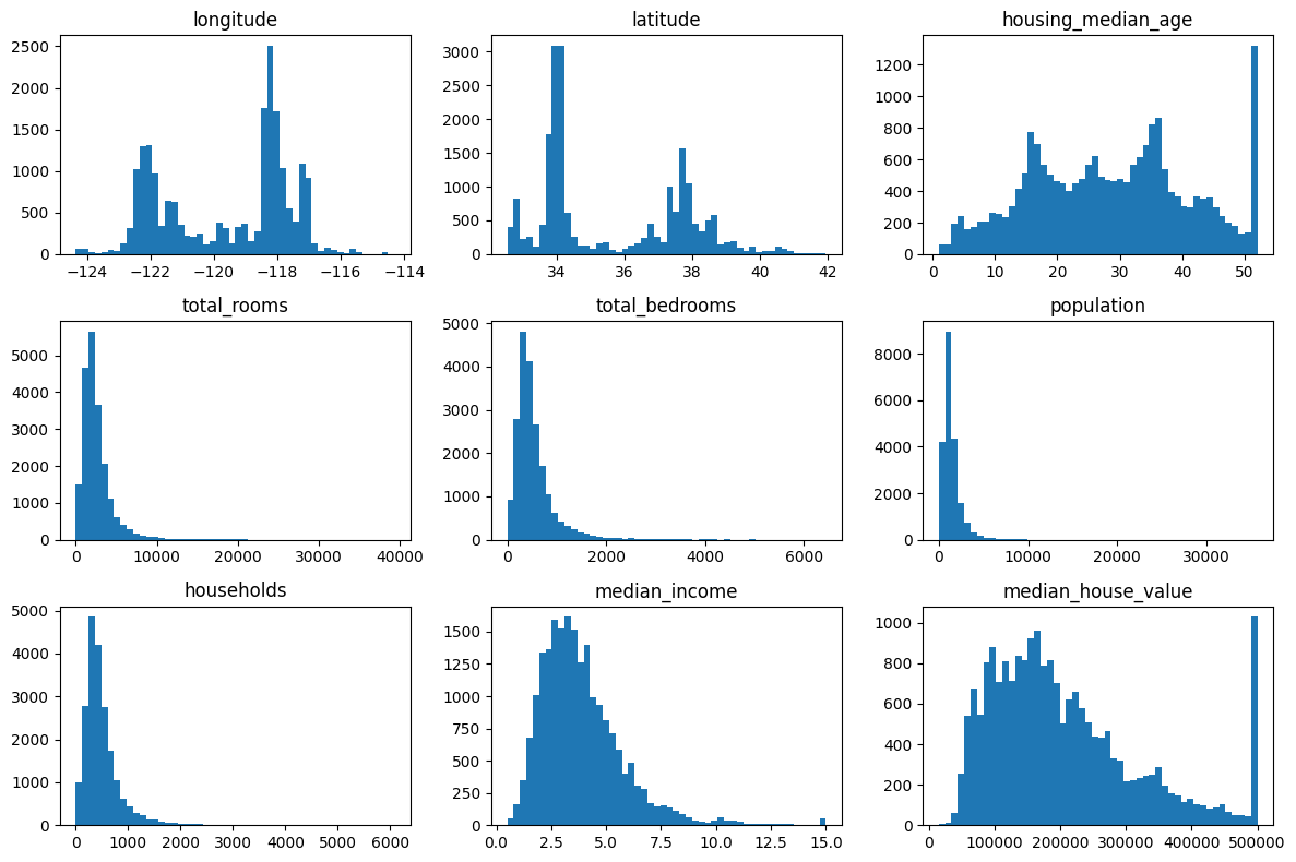

Crear un conjunto de prueba

import numpy as np

def shuffle_and_split_data(data, test_ratio, rng):
    shuffled_indices = rng.permutation(len(data))
    test_set_size = int(len(data) * test_ratio)
    test_indices = shuffled_indices[:test_set_size]
    train_indices = shuffled_indices[test_set_size:]
    return take_rows(data, train_indices), take_rows(data, test_indices)

Para garantizar que las salidas de este notebook sean las mismas cada vez que lo ejecutamos, debemos fijar la semilla aleatoria:

rng = np.random.default_rng(seed=42)
train_set, test_set = shuffle_and_split_data(housing_full, 0.2, rng)
len(train_set)

len(test_set)

Lamentablemente, esto no garantiza que este notebook produzca exactamente los mismos resultados que en el libro, ya que existen otras posibles fuentes de variación. La más importante es que los algoritmos se ajustan con el tiempo a medida que evolucionan las bibliotecas. Así que tolere algunas diferencias menores: idealmente, la mayoría de las salidas deberían ser iguales o, al menos, estar en el rango esperado.

Nota: otra fuente de aleatoriedad es el orden de los set de Python. Depende de la función hash(), que recibe una “sal” aleatoria cuando Python arranca (esto comenzó en Python 3.3 para prevenir ciertos ataques de denegación de servicio). Para eliminar esta aleatoriedad, la solución es configurar la variable de entorno PYTHONHASHSEED en "0" antes de que Python se inicie. Si lo hace después, no ocurrirá nada. Por suerte, si está ejecutando este notebook en Colab, esa variable ya viene configurada.

from zlib import crc32

def is_id_in_test_set(identifier, test_ratio):
    return crc32(np.int64(identifier)) < test_ratio * 2**32


def split_data_with_id_hash(data, test_ratio, id_column):
    in_test_set = pl.Series(
        "in_test_set",
        [is_id_in_test_set(id_, test_ratio) for id_ in data[id_column].to_list()],
    )
    return data.filter(~in_test_set), data.filter(in_test_set)

housing_with_id = housing_full.with_row_index("index")  # agrega una columna `index`
train_set, test_set = split_data_with_id_hash(housing_with_id, 0.2, "index")

housing_with_id = housing_with_id.with_columns(
    (pl.col("longitude") * 1000 + pl.col("latitude")).alias("id")
)
train_set, test_set = split_data_with_id_hash(housing_with_id, 0.2, "id")

from sklearn.model_selection import train_test_split

def sklearn_split_polars(data, *, test_size, random_state, stratify=None):
    indices = np.arange(len(data))
    stratify_values = None if stratify is None else data[stratify].to_numpy()
    train_indices, test_indices = train_test_split(
        indices,
        test_size=test_size,
        random_state=random_state,
        stratify=stratify_values,
    )
    return take_rows(data, train_indices), take_rows(data, test_indices)


train_set, test_set = sklearn_split_polars(
    housing_full, test_size=0.2, random_state=42
)

test_set["total_bedrooms"].is_null().sum()

housing_full = housing_full.with_columns(
    pl.when(pl.col("median_income") < 1.5)
    .then(1)
    .when(pl.col("median_income") < 3.0)
    .then(2)
    .when(pl.col("median_income") < 4.5)
    .then(3)
    .when(pl.col("median_income") < 6.0)
    .then(4)
    .otherwise(5)
    .alias("income_cat")
)

cat_counts = housing_full.group_by("income_cat").len().sort("income_cat")
plt.bar(cat_counts["income_cat"].to_list(), cat_counts["len"].to_list())
plt.xlabel("Categoría de ingresos")
plt.ylabel("Cantidad de distritos");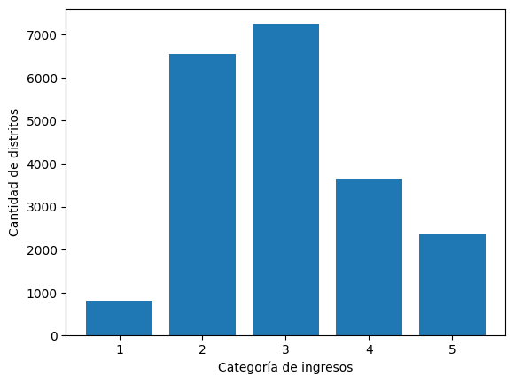

from sklearn.model_selection import StratifiedShuffleSplit

splitter = StratifiedShuffleSplit(n_splits=10, test_size=0.2, random_state=42)
strat_splits = []
for train_index, test_index in splitter.split(
    np.zeros(len(housing_full)), housing_full["income_cat"].to_numpy()
):
    strat_train_set_n = take_rows(housing_full, train_index)
    strat_test_set_n = take_rows(housing_full, test_index)
    strat_splits.append([strat_train_set_n, strat_test_set_n])

strat_train_set, strat_test_set = strat_splits[0]

Es mucho más corto obtener una única partición estratificada:

strat_train_set, strat_test_set = sklearn_split_polars(
    housing_full, test_size=0.2, random_state=42, stratify="income_cat"
)

(
    strat_test_set.group_by("income_cat")
    .len()
    .sort("income_cat")
    .with_columns((pl.col("len") / len(strat_test_set)).alias("proportion"))
    .select("income_cat", "proportion")
)

shape: (5, 2)

income_cat	proportion
i32	f64
1	0.039486
2	0.317345
3	0.35126
4	0.176841
5	0.115068

strat_train_set = strat_train_set.drop("income_cat")
strat_test_set = strat_test_set.drop("income_cat")

Explorar y visualizar los datos para obtener insights

housing = strat_train_set.clone()

Visualización de datos geográficos

plot_scatter(housing, "longitude", "latitude", grid=True);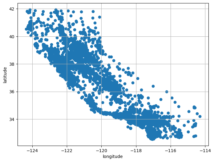

plot_scatter(housing, "longitude", "latitude", grid=True, alpha=0.2);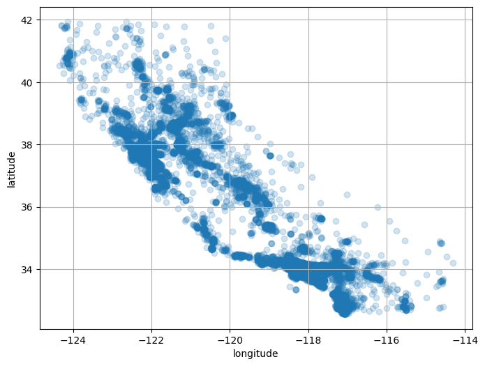

plot_scatter(
    housing,
    "longitude",
    "latitude",
    grid=True,
    s=housing["population"] / 100,
    label="población",
    c=housing["median_house_value"],
    cmap="jet",
    colorbar=True,
    figsize=(10, 7),
);

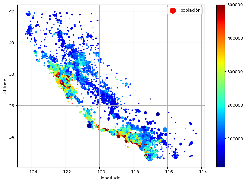
La siguiente celda genera la primera figura del capítulo (este código no está en el libro). Es simplemente una versión mejorada de la figura anterior, con una imagen de California agregada al fondo, etiquetas más agradables y sin grilla.

# Descargar la imagen de California
filename = "california.png"
filepath = Path(f"my_{filename}")
if not filepath.is_file():
    homlp_root = "https://github.com/ageron/handson-mlp/raw/main/"
    url = homlp_root + "images/end_to_end_project/" + filename
    print("Descargando", filename)
    urllib.request.urlretrieve(url, filepath)

housing_renamed = housing.rename(
    {
        "latitude": "Latitud",
        "longitude": "Longitud",
        "population": "Población",
        "median_house_value": "Valor mediano de la vivienda (USD)",
    }
)
plot_scatter(
    housing_renamed,
    "Longitud",
    "Latitud",
    s=housing_renamed["Población"] / 100,
    label="Población",
    c=housing_renamed["Valor mediano de la vivienda (USD)"],
    cmap="jet",
    colorbar=True,
    figsize=(10, 7),
    grid=False,
)

california_img = plt.imread(filepath)
axis = -124.55, -113.95, 32.45, 42.05
plt.axis(axis)
plt.imshow(california_img, extent=axis);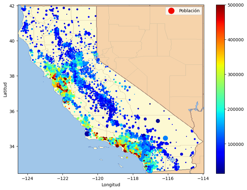

Buscar correlaciones

corr_matrix = housing.select(pl.selectors.numeric()).corr()

pl.DataFrame(
    {
        "atributo": corr_matrix.columns,
        "median_house_value": corr_matrix["median_house_value"],
    }
).sort("median_house_value", descending=True)

shape: (9, 2)

atributo	median_house_value
str	f64
"total_bedrooms"	NaN
"median_house_value"	1.0
"median_income"	0.687369
"total_rooms"	0.132973
"housing_median_age"	0.107244
"households"	0.066395
"population"	-0.025966
"longitude"	-0.049937
"latitude"	-0.14229

attributes = [
    "median_house_value",
    "median_income",
    "total_rooms",
    "housing_median_age",
]
plot_scatter_matrix(housing, attributes, figsize=(12, 8));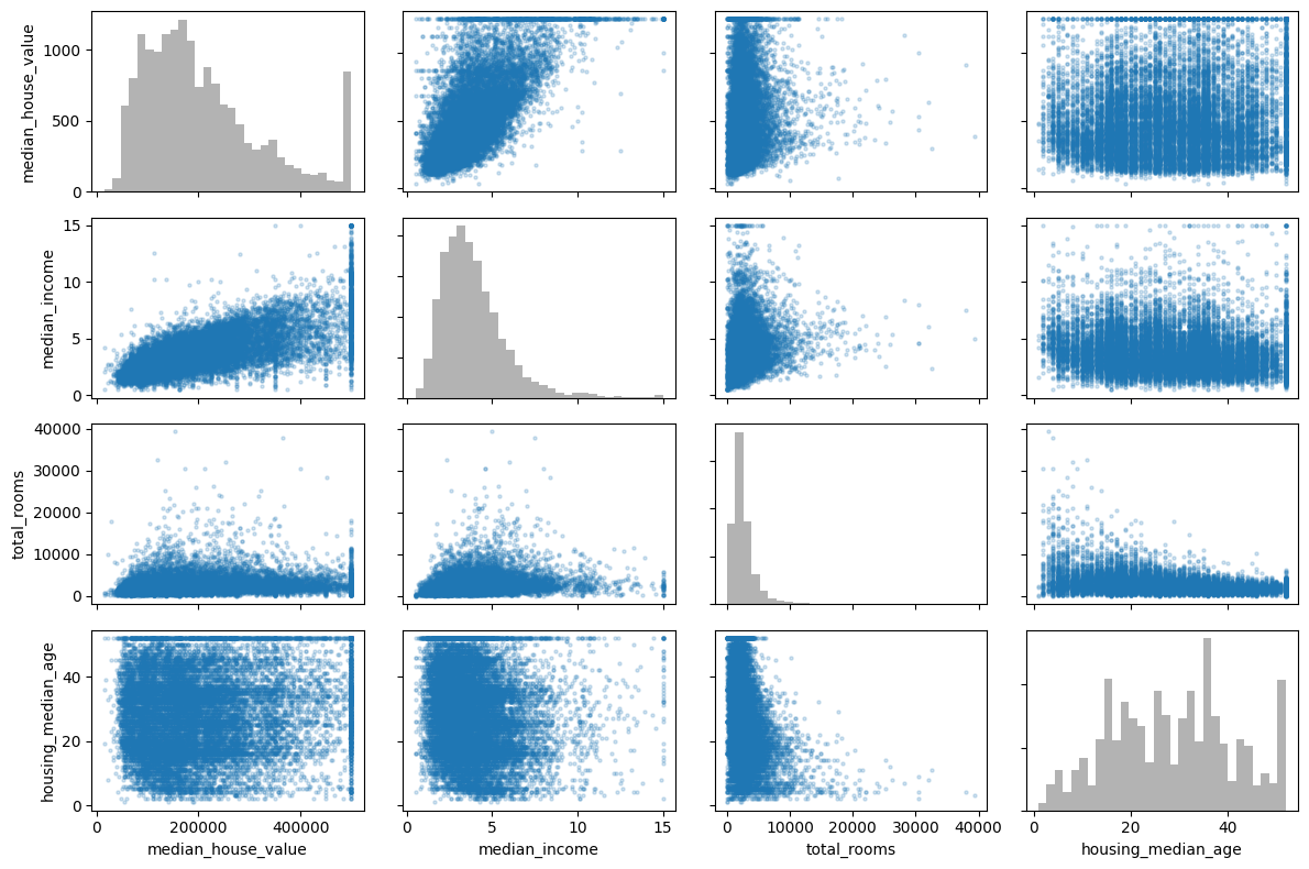

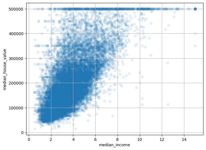
plot_scatter(
    housing,
    "median_income",
    "median_house_value",
    alpha=0.1,
    grid=True,
);

Experimentar con combinaciones de atributos

housing = housing.with_columns(
    (pl.col("total_rooms") / pl.col("households")).alias("rooms_per_house"),
    (pl.col("total_bedrooms") / pl.col("total_rooms")).alias("bedrooms_ratio"),
    (pl.col("population") / pl.col("households")).alias("people_per_house"),
)

corr_matrix = housing.select(pl.selectors.numeric()).corr()
pl.DataFrame(
    {
        "atributo": corr_matrix.columns,
        "median_house_value": corr_matrix["median_house_value"],
    }
).sort("median_house_value", descending=True)

shape: (12, 2)

atributo	median_house_value
str	f64
"total_bedrooms"	NaN
"bedrooms_ratio"	NaN
"median_house_value"	1.0
"median_income"	0.687369
"rooms_per_house"	0.151071
…	…
"households"	0.066395
"people_per_house"	-0.022334
"population"	-0.025966
"longitude"	-0.049937
"latitude"	-0.14229

Preparar los datos para algoritmos de Machine Learning

Volvamos al conjunto de entrenamiento original y separemos la variable objetivo (observe que strat_train_set.drop() crea una copia de strat_train_set sin la columna; no modifica realmente strat_train_set, a menos que pase inplace=True):

housing = strat_train_set.drop("median_house_value")
housing_labels = strat_train_set["median_house_value"].clone()

Nota: la celda anterior reinicia el dataframe housing, eliminando también los atributos personalizados que acabamos de agregar. Hacemos esto porque, más adelante en el capítulo, construiremos un transformation pipeline automatizado para manejar todos estos pasos de una sola vez.

Limpieza de datos

En el libro se enumeran 3 opciones para manejar los valores NaN:

housing = housing.drop_nulls(subset=["total_bedrooms"])  # opción 1

housing = housing.drop("total_bedrooms")  # opción 2

median = housing["total_bedrooms"].median()  # opción 3
housing = housing.with_columns(pl.col("total_bedrooms").fill_null(median))

Para cada opción, crearemos una copia de housing y trabajaremos sobre esa copia para evitar romper housing.

housing_with_row_id = housing.with_row_index("row_id")
null_rows = housing_with_row_id.filter(
    pl.any_horizontal(pl.all().exclude("row_id").is_null())
)
null_row_ids = null_rows["row_id"]
null_rows.head()

shape: (5, 10)

row_id	longitude	latitude	housing_median_age	total_rooms	total_bedrooms	population	households	median_income	ocean_proximity
u32	f64	f64	f64	f64	f64	f64	f64	f64	str
146	-118.27	34.04	13.0	1784.0	null	2158.0	682.0	1.7038	"<1H OCEAN"
263	-117.65	34.04	15.0	3393.0	null	2039.0	611.0	3.9336	"INLAND"
294	-122.5	37.75	44.0	1819.0	null	1137.0	354.0	3.4919	"NEAR OCEAN"
402	-114.59	34.83	41.0	812.0	null	375.0	158.0	1.7083	"INLAND"
411	-118.08	33.92	38.0	1335.0	null	1011.0	269.0	3.6908	"<1H OCEAN"

from sklearn.impute import SimpleImputer

imputer = SimpleImputer(strategy="median")

Separamos los atributos numéricos para usar la estrategia "median" (ya que no puede calcularse sobre atributos de texto como ocean_proximity):

housing_num = housing.select(pl.selectors.numeric())

imputer.fit(housing_num)

SimpleImputer(strategy='median')

In a Jupyter environment, please rerun this cell to show the HTML representation or trust the notebook.
On GitHub, the HTML representation is unable to render, please try loading this page with nbviewer.org.

imputer.statistics_

array([-118.5   ,   34.26  ,   29.    , 2126.5   ,  435.    , 1167.    ,
        410.    ,    3.5394])

Verifiquemos que esto sea lo mismo que calcular manualmente la mediana de cada atributo:

housing_num.median().to_numpy().ravel()

array([-118.5   ,   34.26  ,   29.    , 2126.5   ,  435.    , 1167.    ,
        410.    ,    3.5394])

Transformar el conjunto de entrenamiento:

X = imputer.transform(housing_num)

imputer.feature_names_in_

array(['longitude', 'latitude', 'housing_median_age', 'total_rooms',
       'total_bedrooms', 'population', 'households', 'median_income'],
      dtype=object)

housing_tr = pl.DataFrame(X, schema=housing_num.columns)

(
    housing_tr.with_row_index("row_id")
    .filter(pl.col("row_id").is_in(null_row_ids.to_list()))
    .drop("row_id")
    .head()
)

shape: (5, 8)

longitude	latitude	housing_median_age	total_rooms	total_bedrooms	population	households	median_income
f64	f64	f64	f64	f64	f64	f64	f64
-118.27	34.04	13.0	1784.0	435.0	2158.0	682.0	1.7038
-117.65	34.04	15.0	3393.0	435.0	2039.0	611.0	3.9336
-122.5	37.75	44.0	1819.0	435.0	1137.0	354.0	3.4919
-114.59	34.83	41.0	812.0	435.0	375.0	158.0	1.7083
-118.08	33.92	38.0	1335.0	435.0	1011.0	269.0	3.6908

imputer.strategy

'median'

Ahora descartemos algunos outliers:

from sklearn.ensemble import IsolationForest

isolation_forest = IsolationForest(random_state=42)
outlier_pred = isolation_forest.fit_predict(X)

outlier_pred

array([-1, -1,  1, ...,  1,  1,  1], shape=(16512,))

Si quisiera eliminar outliers, ejecutaría el siguiente código:

# housing = housing.filter(pl.Series("is_inlier", outlier_pred == 1))
# housing_labels = housing_labels.filter(pl.Series("is_inlier", outlier_pred == 1))

Manejo de atributos de texto y categóricos

Ahora preprocesemos la variable de entrada categórica ocean_proximity:

housing_cat = housing.select("ocean_proximity")
housing_cat.head(8)

shape: (8, 1)

ocean_proximity
str
"NEAR BAY"
"NEAR BAY"
"NEAR BAY"
"NEAR BAY"
"NEAR BAY"
"NEAR BAY"
"NEAR BAY"
"NEAR BAY"

from sklearn.preprocessing import OrdinalEncoder

ordinal_encoder = OrdinalEncoder()
housing_cat_encoded = ordinal_encoder.fit_transform(housing_cat)

housing_cat_encoded[:8]

array([[3.],
       [3.],
       [3.],
       [3.],
       [3.],
       [3.],
       [3.],
       [3.]])

ordinal_encoder.categories_

[array(['<1H OCEAN', 'INLAND', 'ISLAND', 'NEAR BAY', 'NEAR OCEAN'],
       dtype=object)]

from sklearn.preprocessing import OneHotEncoder

cat_encoder = OneHotEncoder()
housing_cat_1hot = cat_encoder.fit_transform(housing_cat)

housing_cat_1hot

<Compressed Sparse Row sparse matrix of dtype 'float64'
    with 16512 stored elements and shape (16512, 5)>

Por defecto, la clase OneHotEncoder devuelve un arreglo disperso (sparse), pero podemos convertirlo en un arreglo denso si hace falta llamando al método toarray():

housing_cat_1hot.toarray()

array([[0., 0., 0., 1., 0.],
       [0., 0., 0., 1., 0.],
       [0., 0., 0., 1., 0.],
       ...,
       [0., 1., 0., 0., 0.],
       [0., 1., 0., 0., 0.],
       [0., 1., 0., 0., 0.]], shape=(16512, 5))

Como alternativa, puede establecer sparse_output=False al crear el OneHotEncoder (nota: el hiperparámetro sparse pasó a llamarse sparse_output en Scikit-Learn 1.2):

cat_encoder = OneHotEncoder(sparse_output=False)
housing_cat_1hot = cat_encoder.fit_transform(housing_cat)
housing_cat_1hot

array([[0., 0., 0., 1., 0.],
       [0., 0., 0., 1., 0.],
       [0., 0., 0., 1., 0.],
       ...,
       [0., 1., 0., 0., 0.],
       [0., 1., 0., 0., 0.],
       [0., 1., 0., 0., 0.]], shape=(16512, 5))

cat_encoder.categories_

[array(['<1H OCEAN', 'INLAND', 'ISLAND', 'NEAR BAY', 'NEAR OCEAN'],
       dtype=object)]

df_test = pl.DataFrame({"ocean_proximity": ["INLAND", "NEAR BAY"]})
df_test.to_dummies()

shape: (2, 2)

ocean_proximity_INLAND	ocean_proximity_NEAR BAY
u8	u8
1	0
0	1

cat_encoder.transform(df_test)

array([[0., 1., 0., 0., 0.],
       [0., 0., 0., 1., 0.]])

df_test_unknown = pl.DataFrame({"ocean_proximity": ["<2H OCEAN", "ISLAND"]})
df_test_unknown.to_dummies()

shape: (2, 2)

ocean_proximity_<2H OCEAN	ocean_proximity_ISLAND
u8	u8
1	0
0	1

cat_encoder.handle_unknown = "ignore"
cat_encoder.transform(df_test_unknown)

array([[0., 0., 0., 0., 0.],
       [0., 0., 1., 0., 0.]])

cat_encoder.feature_names_in_

array(['ocean_proximity'], dtype=object)

cat_encoder.get_feature_names_out()

array(['ocean_proximity_<1H OCEAN', 'ocean_proximity_INLAND',
       'ocean_proximity_ISLAND', 'ocean_proximity_NEAR BAY',
       'ocean_proximity_NEAR OCEAN'], dtype=object)

cat_encoder.transform(df_test_unknown)

array([[0., 0., 0., 0., 0.],
       [0., 0., 1., 0., 0.]])

df_output = pl.DataFrame(
    cat_encoder.transform(df_test_unknown),
    schema=list(cat_encoder.get_feature_names_out()),
)

df_output

shape: (2, 5)

ocean_proximity_<1H OCEAN	ocean_proximity_INLAND	ocean_proximity_ISLAND	ocean_proximity_NEAR BAY	ocean_proximity_NEAR OCEAN
f64	f64	f64	f64	f64
0.0	0.0	0.0	0.0	0.0
0.0	0.0	1.0	0.0	0.0

Escalado de atributos

from sklearn.preprocessing import MinMaxScaler

min_max_scaler = MinMaxScaler(feature_range=(-1, 1))
housing_num_min_max_scaled = min_max_scaler.fit_transform(housing_num)

from sklearn.preprocessing import StandardScaler

std_scaler = StandardScaler()
housing_num_std_scaled = std_scaler.fit_transform(housing_num)

# código extra – esta celda genera la Figura 2–17
fig, axs = plt.subplots(1, 2, figsize=(8, 3), sharey=True)
axs[0].hist(housing["population"].drop_nulls().to_numpy(), bins=50)
axs[1].hist(np.log(housing["population"].drop_nulls().to_numpy()), bins=50)
axs[0].set_xlabel("Población")
axs[1].set_xlabel("Logaritmo de la población")
axs[0].set_ylabel("Cantidad de distritos");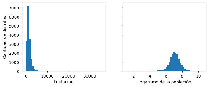

from sklearn.metrics.pairwise import rbf_kernel

age_simil_35 = rbf_kernel(
    housing.select("housing_median_age").to_numpy(), [[35]], gamma=0.1
)

# código extra – esta celda genera la Figura 2–18

ages = np.linspace(
    housing["housing_median_age"].min(), housing["housing_median_age"].max(), 500
).reshape(-1, 1)
gamma1 = 0.1
gamma2 = 0.03
rbf1 = rbf_kernel(ages, [[35]], gamma=gamma1)
rbf2 = rbf_kernel(ages, [[35]], gamma=gamma2)

fig, ax1 = plt.subplots()

ax1.set_xlabel("Antigüedad mediana de las viviendas")
ax1.set_ylabel("Cantidad de distritos")
ax1.hist(housing["housing_median_age"].drop_nulls().to_numpy(), bins=50)

ax2 = ax1.twinx()  # crear un eje gemelo que comparta el mismo eje x
color = "blue"
ax2.plot(ages, rbf1, color=color, label="gamma = 0.10")
ax2.plot(ages, rbf2, color=color, label="gamma = 0.03", linestyle="--")
ax2.tick_params(axis="y", labelcolor=color)
ax2.set_ylabel("Similitud de antigüedad", color=color)

plt.legend(loc="upper left")

plt.show()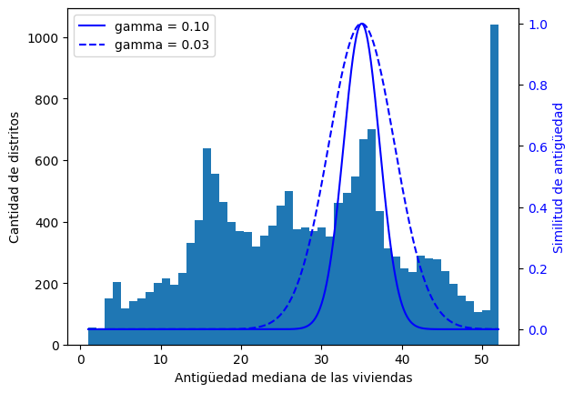

from sklearn.linear_model import LinearRegression

target_scaler = StandardScaler()
scaled_labels = target_scaler.fit_transform(housing_labels.to_frame().to_numpy())

model = LinearRegression()
model.fit(housing.select("median_income").to_numpy(), scaled_labels)
some_new_data = housing.select("median_income").head(5)  # supongamos que estos son datos nuevos

scaled_predictions = model.predict(some_new_data.to_numpy())
predictions = target_scaler.inverse_transform(scaled_predictions)

predictions

array([[393767.28579276],
       [392768.19727172],
       [348942.63357583],
       [281176.72603341],
       [205745.54269514]])

from sklearn.compose import TransformedTargetRegressor

model = TransformedTargetRegressor(LinearRegression(), transformer=StandardScaler())
model.fit(housing.select("median_income").to_numpy(), housing_labels.to_numpy())
predictions = model.predict(some_new_data.to_numpy())

predictions

array([393767.28579276, 392768.19727172, 348942.63357583, 281176.72603341,
       205745.54269514])

Transformadores personalizados

Para crear transformadores simples:

from sklearn.preprocessing import FunctionTransformer

log_transformer = FunctionTransformer(np.log, inverse_func=np.exp)
log_pop = log_transformer.transform(housing.select("population").to_numpy())

rbf_transformer = FunctionTransformer(rbf_kernel, kw_args=dict(Y=[[35.0]], gamma=0.1))
age_simil_35 = rbf_transformer.transform(housing.select("housing_median_age").to_numpy())

age_simil_35

array([[2.73237224e-02],
       [3.07487988e-09],
       [2.81118530e-13],
       ...,
       [2.81118530e-13],
       [2.81118530e-13],
       [2.09879105e-16]], shape=(16512, 1))

sf_coords = 37.7749, -122.41
sf_transformer = FunctionTransformer(rbf_kernel, kw_args=dict(Y=[sf_coords], gamma=0.1))
sf_simil = sf_transformer.transform(
    housing.select("latitude", "longitude").to_numpy()
)

sf_simil

array([[0.99566482],
       [0.99567518],
       [0.99655196],
       ...,
       [0.6452246 ],
       [0.6752005 ],
       [0.67616077]], shape=(16512, 1))

ratio_transformer = FunctionTransformer(lambda X: X[:, [0]] / X[:, [1]])
ratio_transformer.transform(np.array([[1.0, 2.0], [3.0, 4.0]]))

array([[0.5 ],
       [0.75]])

from sklearn.base import BaseEstimator, TransformerMixin
from sklearn.utils.validation import check_array, check_is_fitted


class StandardScalerClone(BaseEstimator, TransformerMixin):
    def __init__(self, with_mean=True):  # sin *args ni **kwargs
        self.with_mean = with_mean

    def fit(self, X, y=None):  # y es obligatorio aunque no lo usemos
        X = check_array(X)  # verifica que X sea un arreglo con valores float finitos
        self.mean_ = X.mean(axis=0)
        self.scale_ = X.std(axis=0)
        self.n_features_in_ = X.shape[1]  # todo estimador guarda esto en fit()
        return self  # siempre devolver self

    def transform(self, X):
        check_is_fitted(self)  # busca atributos aprendidos (terminados en _)
        X = check_array(X)
        assert self.n_features_in_ == X.shape[1]
        if self.with_mean:
            X = X - self.mean_
        return X / self.scale_

from sklearn.cluster import KMeans


class ClusterSimilarity(BaseEstimator, TransformerMixin):
    def __init__(self, n_clusters=10, gamma=1.0, random_state=None):
        self.n_clusters = n_clusters
        self.gamma = gamma
        self.random_state = random_state

    def fit(self, X, y=None, sample_weight=None):
        self.kmeans_ = KMeans(self.n_clusters, random_state=self.random_state)
        self.kmeans_.fit(X, sample_weight=sample_weight)
        return self  # siempre devolver self

    def transform(self, X):
        return rbf_kernel(X, self.kmeans_.cluster_centers_, gamma=self.gamma)

    def get_feature_names_out(self, names=None):
        return [f"Similitud con cluster {i}" for i in range(self.n_clusters)]

Agrupemos los distritos basándonos solo en la latitud y la longitud:

cluster_simil = ClusterSimilarity(n_clusters=10, gamma=1.0, random_state=42)
similarities = cluster_simil.fit_transform(
    housing.select("latitude", "longitude").to_numpy()
)

similarities[:3].round(2)

array([[0.27, 0.  , 0.  , 0.  , 0.76, 0.03, 0.87, 0.  , 0.  , 0.  ],
       [0.28, 0.  , 0.  , 0.  , 0.74, 0.03, 0.89, 0.  , 0.  , 0.  ],
       [0.26, 0.  , 0.  , 0.  , 0.74, 0.03, 0.89, 0.  , 0.  , 0.  ]])

housing = strat_train_set.clone()

# código extra – esta celda genera la Figura 2–19

housing_renamed = housing.rename(
    {
        "latitude": "Latitud",
        "longitude": "Longitud",
        "population": "Población",
        "median_house_value": "Valor mediano de la vivienda (USD)",
    }
)
housing_renamed = housing_renamed.with_columns(
    pl.Series("Similitud máxima con cluster", similarities.max(axis=1))
)

plot_scatter(
    housing_renamed,
    "Longitud",
    "Latitud",
    grid=True,
    s=housing_renamed["Población"] / 100,
    label="Población",
    c=housing_renamed["Similitud máxima con cluster"],
    cmap="jet",
    colorbar=True,
    figsize=(10, 7),
)
plt.plot(
    cluster_simil.kmeans_.cluster_centers_[:, 1],
    cluster_simil.kmeans_.cluster_centers_[:, 0],
    linestyle="",
    color="black",
    marker="X",
    markersize=20,
    label="Centros de cluster",
)
plt.legend(loc="upper right")

plt.show()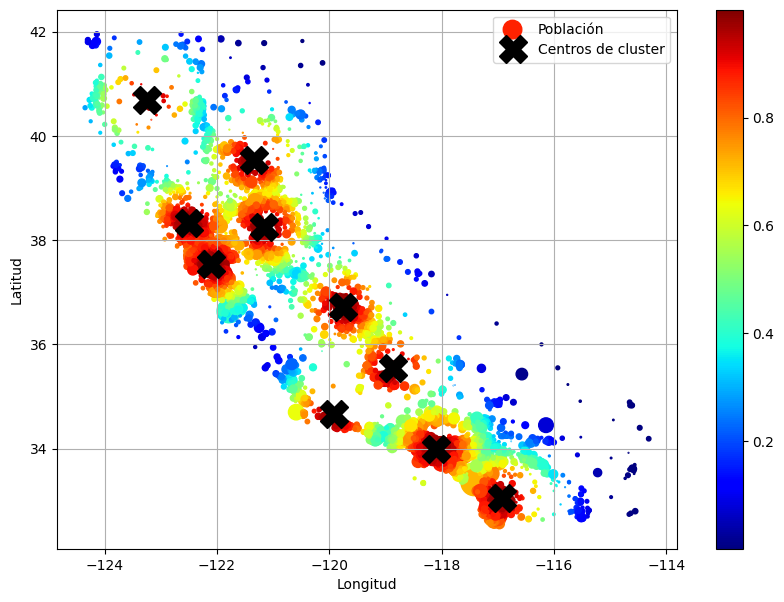

housing = strat_train_set.drop("median_house_value")

Pipelines de transformación

Ahora construyamos un pipeline para preprocesar los atributos numéricos:

from sklearn.pipeline import Pipeline

num_pipeline = Pipeline(
    [
        ("impute", SimpleImputer(strategy="median")),
        ("standardize", StandardScaler()),
    ]
)

from sklearn.pipeline import make_pipeline

num_pipeline = make_pipeline(SimpleImputer(strategy="median"), StandardScaler())

from sklearn import set_config

set_config(display="diagram")

num_pipeline

Pipeline(steps=[('simpleimputer', SimpleImputer(strategy='median')),
                ('standardscaler', StandardScaler())])

housing_num_prepared = num_pipeline.fit_transform(housing_num)
housing_num_prepared[:2].round(2)

array([[-1.33,  1.05,  0.99, -0.8 , -0.97, -0.96, -0.97,  2.36],
       [-1.32,  1.04, -0.6 ,  2.03,  1.35,  0.85,  1.67,  2.34]])

df_housing_num_prepared = pl.DataFrame(
    housing_num_prepared,
    schema=list(num_pipeline.get_feature_names_out()),
)

df_housing_num_prepared.head(2)  # código extra

shape: (2, 8)

longitude	latitude	housing_median_age	total_rooms	total_bedrooms	population	households	median_income
f64	f64	f64	f64	f64	f64	f64	f64
-1.327964	1.050099	0.98585	-0.796827	-0.965763	-0.964302	-0.973804	2.357306
-1.322969	1.040734	-0.604307	2.026566	1.35019	0.851473	1.670428	2.344717

num_pipeline.steps

[('simpleimputer', SimpleImputer(strategy='median')),
 ('standardscaler', StandardScaler())]

num_pipeline[1]

StandardScaler()

num_pipeline[:-1]

Pipeline(steps=[('simpleimputer', SimpleImputer(strategy='median'))])

num_pipeline.named_steps["simpleimputer"]

SimpleImputer(strategy='median')

num_pipeline.set_params(simpleimputer__strategy="median")

Pipeline(steps=[('simpleimputer', SimpleImputer(strategy='median')),
                ('standardscaler', StandardScaler())])

from sklearn.compose import ColumnTransformer

num_attribs = [
    "longitude",
    "latitude",
    "housing_median_age",
    "total_rooms",
    "total_bedrooms",
    "population",
    "households",
    "median_income",
]
cat_attribs = ["ocean_proximity"]

cat_pipeline = make_pipeline(
    SimpleImputer(strategy="most_frequent"), OneHotEncoder(handle_unknown="ignore")
)

preprocessing = ColumnTransformer(
    [
        ("num", num_pipeline, num_attribs),
        ("cat", cat_pipeline, cat_attribs),
    ]
)

from sklearn.compose import make_column_transformer


def numeric_columns(df):
    return df.select(pl.selectors.numeric()).columns


def string_columns(df):
    return df.select(pl.col(pl.String)).columns


preprocessing = make_column_transformer(
    (num_pipeline, numeric_columns),
    (cat_pipeline, string_columns),
)

housing_prepared = preprocessing.fit_transform(housing)

# código extra – muestra que podemos obtener un DataFrame si queremos
housing_prepared_fr = pl.DataFrame(
    housing_prepared,
    schema=list(preprocessing.get_feature_names_out()),
)
housing_prepared_fr.head(2)

shape: (2, 13)

pipeline-1__longitude	pipeline-1__latitude	pipeline-1__housing_median_age	pipeline-1__total_rooms	pipeline-1__total_bedrooms	pipeline-1__population	pipeline-1__households	pipeline-1__median_income	pipeline-2__ocean_proximity_<1H OCEAN	pipeline-2__ocean_proximity_INLAND	pipeline-2__ocean_proximity_ISLAND	pipeline-2__ocean_proximity_NEAR BAY	pipeline-2__ocean_proximity_NEAR OCEAN
f64	f64	f64	f64	f64	f64	f64	f64	f64	f64	f64	f64	f64
-1.327964	1.050099	0.98585	-0.796827	-0.965763	-0.964302	-0.973804	2.357306	0.0	0.0	0.0	1.0	0.0
-1.322969	1.040734	-0.604307	2.026566	1.35019	0.851473	1.670428	2.344717	0.0	0.0	0.0	1.0	0.0

def column_ratio(X):
    return X[:, [0]] / X[:, [1]]


def ratio_name(function_transformer, feature_names_in):
    return ["ratio"]  # nombres de atributos de salida

def ratio_pipeline():
    return make_pipeline(
        SimpleImputer(strategy="median"),
        FunctionTransformer(column_ratio, feature_names_out=ratio_name),
        StandardScaler(),
    )

log_pipeline = make_pipeline(
    SimpleImputer(strategy="median"),
    FunctionTransformer(np.log, feature_names_out="one-to-one"),
    StandardScaler(),
)

cluster_simil = ClusterSimilarity(n_clusters=10, gamma=1.0, random_state=42)
default_num_pipeline = make_pipeline(SimpleImputer(strategy="median"), StandardScaler())
preprocessing = ColumnTransformer(
    [
        ("bedrooms", ratio_pipeline(), ["total_bedrooms", "total_rooms"]),
        ("rooms_per_house", ratio_pipeline(), ["total_rooms", "households"]),
        ("people_per_house", ratio_pipeline(), ["population", "households"]),
        (
            "log",
            log_pipeline,
            [
                "total_bedrooms",
                "total_rooms",
                "population",
                "households",
                "median_income",
            ],
        ),
        ("geo", cluster_simil, ["latitude", "longitude"]),
        ("cat", cat_pipeline, string_columns),
    ],
    remainder=default_num_pipeline,
)  # queda una columna: housing_median_age

housing_prepared = preprocessing.fit_transform(housing)
housing_prepared.shape

(16512, 24)

preprocessing.get_feature_names_out()

array(['bedrooms__ratio', 'rooms_per_house__ratio',
       'people_per_house__ratio', 'log__total_bedrooms',
       'log__total_rooms', 'log__population', 'log__households',
       'log__median_income', 'geo__Similitud con cluster 0',
       'geo__Similitud con cluster 1', 'geo__Similitud con cluster 2',
       'geo__Similitud con cluster 3', 'geo__Similitud con cluster 4',
       'geo__Similitud con cluster 5', 'geo__Similitud con cluster 6',
       'geo__Similitud con cluster 7', 'geo__Similitud con cluster 8',
       'geo__Similitud con cluster 9', 'cat__ocean_proximity_<1H OCEAN',
       'cat__ocean_proximity_INLAND', 'cat__ocean_proximity_ISLAND',
       'cat__ocean_proximity_NEAR BAY', 'cat__ocean_proximity_NEAR OCEAN',
       'remainder__housing_median_age'], dtype=object)

Seleccionar y entrenar un modelo

Entrenar y evaluar sobre el conjunto de entrenamiento

from sklearn.linear_model import LinearRegression

lin_reg = make_pipeline(preprocessing, LinearRegression())
lin_reg.fit(housing, housing_labels.to_numpy())

Probemos el pipeline completo de preprocessing sobre algunas instancias de entrenamiento:

housing_predictions = lin_reg.predict(housing)
housing_predictions[:5].round(-2)  # -2 = redondeado al centenar más cercano

array([367300., 374600., 359000., 319200., 292000.])

Comparemos con los valores reales:

housing_labels.head(5).to_numpy()

array([452600., 358500., 352100., 341300., 342200.])

# código extra – calcula las razones de error discutidas en el libro
error_ratios = housing_predictions[:5].round(-2) / housing_labels.head(5).to_numpy() - 1
print(", ".join([f"{100 * ratio:.1f}%" for ratio in error_ratios]))

-18.8%, 4.5%, 2.0%, -6.5%, -14.7%

from sklearn.metrics import root_mean_squared_error

lin_rmse = root_mean_squared_error(housing_labels.to_numpy(), housing_predictions)
lin_rmse

69628.72473814597

from sklearn.tree import DecisionTreeRegressor

tree_reg = make_pipeline(preprocessing, DecisionTreeRegressor(random_state=42))
tree_reg.fit(housing, housing_labels.to_numpy())

housing_predictions = tree_reg.predict(housing)
tree_rmse = root_mean_squared_error(housing_labels.to_numpy(), housing_predictions)
tree_rmse

0.0

Mejor evaluación mediante cross-validation

from sklearn.model_selection import cross_val_score

tree_rmses = -cross_val_score(
    tree_reg,
    housing,
    housing_labels.to_numpy(),
    scoring="neg_root_mean_squared_error",
    cv=10,
)

pl.Series("tree_rmses", tree_rmses).describe()

shape: (9, 2)

statistic	value
str	f64
"count"	10.0
"null_count"	0.0
"mean"	66503.04337
"std"	3049.595021
"min"	63208.146847
"25%"	64161.106398
"50%"	65851.915768
"75%"	69152.616327
"max"	71977.004064

# código extra – calcula las estadísticas de error para el modelo lineal
lin_rmses = -cross_val_score(
    lin_reg,
    housing,
    housing_labels.to_numpy(),
    scoring="neg_root_mean_squared_error",
    cv=10,
)
pl.Series("lin_rmses", lin_rmses).describe()

shape: (9, 2)

statistic	value
str	f64
"count"	10.0
"null_count"	0.0
"mean"	70705.192866
"std"	4890.581493
"min"	66050.489442
"25%"	68065.090371
"50%"	70038.330666
"75%"	70411.493896
"max"	83156.970571

Advertencia: la siguiente celda puede tardar algunos minutos en ejecutarse:

from sklearn.ensemble import RandomForestRegressor

forest_reg = make_pipeline(preprocessing, RandomForestRegressor(random_state=42))
forest_rmses = -cross_val_score(
    forest_reg,
    housing,
    housing_labels.to_numpy(),
    scoring="neg_root_mean_squared_error",
    cv=10,
)

pl.Series("forest_rmses", forest_rmses).describe()

shape: (9, 2)

statistic	value
str	f64
"count"	10.0
"null_count"	0.0
"mean"	47327.917283
"std"	2120.353226
"min"	44296.059343
"25%"	45157.740907
"50%"	47659.703366
"75%"	48574.14477
"max"	51156.913725

Comparemos este RMSE medido con cross-validation (el “error de validación”) con el RMSE medido sobre el conjunto de entrenamiento (el “error de entrenamiento”):

forest_reg.fit(housing, housing_labels.to_numpy())
housing_predictions = forest_reg.predict(housing)
forest_rmse = root_mean_squared_error(housing_labels.to_numpy(), housing_predictions)
forest_rmse

17544.565814894762

El error de entrenamiento es mucho más bajo que el error de validación, lo que normalmente significa que el modelo hizo overfitting sobre el conjunto de entrenamiento. Otra posible explicación sería que existe un desajuste entre los datos de entrenamiento y los de validación, pero no es el caso aquí, ya que ambos provienen del mismo dataset que mezclamos y dividimos en dos partes.

Ajustar finamente el modelo

Grid search

Advertencia: la siguiente celda puede tardar algunos minutos en ejecutarse:

from sklearn.model_selection import GridSearchCV

full_pipeline = Pipeline(
    [
        ("preprocessing", preprocessing),
        ("random_forest", RandomForestRegressor(random_state=42)),
    ]
)
param_grid = [
    {
        "preprocessing__geo__n_clusters": [5, 8, 10],
        "random_forest__max_features": [4, 6, 8],
    },
    {
        "preprocessing__geo__n_clusters": [10, 15],
        "random_forest__max_features": [6, 8, 10],
    },
]
grid_search = GridSearchCV(
    full_pipeline, param_grid, cv=3, scoring="neg_root_mean_squared_error"
)
grid_search.fit(housing, housing_labels.to_numpy())

Puede obtener la lista completa de hiperparámetros disponibles para ajustar consultando full_pipeline.get_params().keys():

# código extra – muestra parte de la salida de get_params().keys()
print(str(full_pipeline.get_params().keys())[:1000] + "...")

dict_keys(['memory', 'steps', 'transform_input', 'verbose', 'preprocessing', 'random_forest', 'preprocessing__force_int_remainder_cols', 'preprocessing__n_jobs', 'preprocessing__remainder__memory', 'preprocessing__remainder__steps', 'preprocessing__remainder__transform_input', 'preprocessing__remainder__verbose', 'preprocessing__remainder__simpleimputer', 'preprocessing__remainder__standardscaler', 'preprocessing__remainder__simpleimputer__add_indicator', 'preprocessing__remainder__simpleimputer__copy', 'preprocessing__remainder__simpleimputer__fill_value', 'preprocessing__remainder__simpleimputer__keep_empty_features', 'preprocessing__remainder__simpleimputer__missing_values', 'preprocessing__remainder__simpleimputer__strategy', 'preprocessing__remainder__standardscaler__copy', 'preprocessing__remainder__standardscaler__with_mean', 'preprocessing__remainder__standardscaler__with_std', 'preprocessing__remainder', 'preprocessing__sparse_threshold', 'preprocessing__transformer_weights', ...

La mejor combinación de hiperparámetros encontrada:

grid_search.best_params_

{'preprocessing__geo__n_clusters': 15, 'random_forest__max_features': 6}

grid_search.best_estimator_

Veamos la puntuación de cada combinación de hiperparámetros probada durante el grid search:

cv_res = pl.DataFrame(grid_search.cv_results_).sort("mean_test_score", descending=True)

# código extra – estas líneas solo hacen que el DataFrame se vea mejor
cv_res = cv_res.select(
    [
        "param_preprocessing__geo__n_clusters",
        "param_random_forest__max_features",
        "split0_test_score",
        "split1_test_score",
        "split2_test_score",
        "mean_test_score",
    ]
)
score_cols = ["split0", "split1", "split2", "mean_test_rmse"]
cv_res.columns = ["n_clusters", "max_features"] + score_cols
cv_res = cv_res.with_columns(
    [(-pl.col(col)).round(0).cast(pl.Int64).alias(col) for col in score_cols]
)

cv_res.head()

shape: (5, 6)

n_clusters	max_features	split0	split1	split2	mean_test_rmse
i64	i64	i64	i64	i64	i64
15	6	46245	43926	42404	44192
15	8	46333	44255	43159	44582
15	10	46697	44813	43652	45054
10	6	47320	45026	43774	45374
10	6	47320	45026	43774	45374

Randomized search

from sklearn.experimental import enable_halving_search_cv
from sklearn.model_selection import HalvingRandomSearchCV

Probar 30 combinaciones aleatorias de hiperparámetros (n_iter × cv):

Advertencia: la siguiente celda puede tardar algunos minutos en ejecutarse:

from sklearn.model_selection import RandomizedSearchCV
from scipy.stats import randint

param_distribs = {
    "preprocessing__geo__n_clusters": randint(low=3, high=50),
    "random_forest__max_features": randint(low=2, high=20),
}

rnd_search = RandomizedSearchCV(
    full_pipeline,
    param_distributions=param_distribs,
    n_iter=10,
    cv=3,
    scoring="neg_root_mean_squared_error",
    random_state=42,
)

rnd_search.fit(housing, housing_labels.to_numpy())

# código extra – muestra los resultados del randomized search
cv_res = pl.DataFrame(rnd_search.cv_results_).sort("mean_test_score", descending=True)
cv_res = cv_res.select(
    [
        "param_preprocessing__geo__n_clusters",
        "param_random_forest__max_features",
        "split0_test_score",
        "split1_test_score",
        "split2_test_score",
        "mean_test_score",
    ]
)
cv_res.columns = ["n_clusters", "max_features"] + score_cols
cv_res = cv_res.with_columns(
    [(-pl.col(col)).round(0).cast(pl.Int64).alias(col) for col in score_cols]
)
cv_res.head()

shape: (5, 6)

n_clusters	max_features	split0	split1	split2	mean_test_rmse
i64	i64	i64	i64	i64	i64
45	9	44595	42167	41261	42675
32	7	44561	42348	41527	42812
41	16	45101	43004	41610	43238
42	4	45306	42570	41897	43258
23	8	45531	43090	41901	43507

Analizar los mejores modelos y sus errores

final_model = rnd_search.best_estimator_  # incluye preprocessing
feature_importances = final_model["random_forest"].feature_importances_
feature_importances.round(2)

array([0.07, 0.06, 0.05, 0.01, 0.01, 0.01, 0.01, 0.18, 0.01, 0.01, 0.02,
       0.01, 0.  , 0.01, 0.01, 0.02, 0.01, 0.01, 0.01, 0.02, 0.01, 0.01,
       0.01, 0.02, 0.  , 0.02, 0.01, 0.01, 0.01, 0.01, 0.02, 0.01, 0.01,
       0.01, 0.01, 0.01, 0.  , 0.02, 0.02, 0.02, 0.01, 0.01, 0.01, 0.01,
       0.01, 0.01, 0.01, 0.01, 0.04, 0.01, 0.01, 0.01, 0.01, 0.  , 0.07,
       0.  , 0.  , 0.  , 0.01])

sorted(
    zip(feature_importances, final_model["preprocessing"].get_feature_names_out()),
    reverse=True,
)

[(np.float64(0.17880238131149134), 'log__median_income'),
 (np.float64(0.07381749533772475), 'bedrooms__ratio'),
 (np.float64(0.07267469411184849), 'cat__ocean_proximity_INLAND'),
 (np.float64(0.05698858473027031), 'rooms_per_house__ratio'),
 (np.float64(0.05089874665251742), 'people_per_house__ratio'),
 (np.float64(0.0376693387226664), 'geo__Similitud con cluster 40'),
 (np.float64(0.02415140988126297), 'geo__Similitud con cluster 29'),
 (np.float64(0.023056013193885165), 'geo__Similitud con cluster 17'),
 (np.float64(0.022163413185462433), 'geo__Similitud con cluster 2'),
 (np.float64(0.022162257131750136), 'geo__Similitud con cluster 7'),
 (np.float64(0.02042285785093997), 'geo__Similitud con cluster 15'),
 (np.float64(0.01796973985448446), 'geo__Similitud con cluster 11'),
 (np.float64(0.01644197852121045), 'geo__Similitud con cluster 22'),
 (np.float64(0.015231042485248592), 'geo__Similitud con cluster 31'),
 (np.float64(0.015208213770897637), 'geo__Similitud con cluster 30'),
 (np.float64(0.013601365168233286), 'geo__Similitud con cluster 36'),
 (np.float64(0.012879673633151505), 'geo__Similitud con cluster 18'),
 (np.float64(0.012544752224037418), 'geo__Similitud con cluster 38'),
 (np.float64(0.011648403572444874), 'geo__Similitud con cluster 14'),
 (np.float64(0.01126425636603314), 'remainder__housing_median_age'),
 (np.float64(0.011091768428009605), 'geo__Similitud con cluster 6'),
 (np.float64(0.010971499944283033), 'geo__Similitud con cluster 1'),
 (np.float64(0.010863042452808511), 'geo__Similitud con cluster 9'),
 (np.float64(0.010836507704732443), 'geo__Similitud con cluster 33'),
 (np.float64(0.010789603511453758), 'geo__Similitud con cluster 34'),
 (np.float64(0.010704393421761363), 'geo__Similitud con cluster 10'),
 (np.float64(0.010347789523146514), 'geo__Similitud con cluster 19'),
 (np.float64(0.010216904531612496), 'geo__Similitud con cluster 42'),
 (np.float64(0.010106353398536744), 'geo__Similitud con cluster 37'),
 (np.float64(0.0099007536351829), 'geo__Similitud con cluster 32'),
 (np.float64(0.009890071197534054), 'geo__Similitud con cluster 3'),
 (np.float64(0.009868129642864957), 'geo__Similitud con cluster 44'),
 (np.float64(0.009784488666806557), 'geo__Similitud con cluster 41'),
 (np.float64(0.009719992470298493), 'geo__Similitud con cluster 20'),
 (np.float64(0.009428016103346556), 'geo__Similitud con cluster 13'),
 (np.float64(0.008820080231971164), 'geo__Similitud con cluster 24'),
 (np.float64(0.008411986746413521), 'geo__Similitud con cluster 23'),
 (np.float64(0.008074982510801153), 'geo__Similitud con cluster 35'),
 (np.float64(0.008004412241008393), 'geo__Similitud con cluster 25'),
 (np.float64(0.0074611952172112155), 'log__total_rooms'),
 (np.float64(0.0074070095997275836), 'log__population'),
 (np.float64(0.006946890788603158), 'log__total_bedrooms'),
 (np.float64(0.006904926382982712), 'geo__Similitud con cluster 8'),
 (np.float64(0.006852851910228645), 'geo__Similitud con cluster 0'),
 (np.float64(0.006696610040971746), 'geo__Similitud con cluster 43'),
 (np.float64(0.006663835056774162), 'log__households'),
 (np.float64(0.006649407509438607), 'geo__Similitud con cluster 27'),
 (np.float64(0.006640489911985824), 'geo__Similitud con cluster 12'),
 (np.float64(0.006396353239977865), 'geo__Similitud con cluster 5'),
 (np.float64(0.006388870363523759), 'geo__Similitud con cluster 21'),
 (np.float64(0.0055500385351580145), 'geo__Similitud con cluster 26'),
 (np.float64(0.005054627721788298), 'geo__Similitud con cluster 39'),
 (np.float64(0.00470777883759686), 'geo__Similitud con cluster 16'),
 (np.float64(0.004343426620638807), 'geo__Similitud con cluster 28'),
 (np.float64(0.002961318447265596), 'cat__ocean_proximity_<1H OCEAN'),
 (np.float64(0.002479170582746683), 'cat__ocean_proximity_NEAR OCEAN'),
 (np.float64(0.0020286683388693583), 'geo__Similitud con cluster 4'),
 (np.float64(0.0003880798895669554), 'cat__ocean_proximity_NEAR BAY'),
 (np.float64(5.105693681134237e-05), 'cat__ocean_proximity_ISLAND')]

Evaluar el sistema en el conjunto de prueba

X_test = strat_test_set.drop("median_house_value")
y_test = strat_test_set["median_house_value"]

final_predictions = final_model.predict(X_test)

final_rmse = root_mean_squared_error(y_test.to_numpy(), final_predictions)
print(final_rmse)

40623.466919823426

Podemos calcular un intervalo de confianza del 95% para el RMSE de prueba usando la función bootstrap() de SciPy:

from scipy.stats import bootstrap

def rmse(squared_errors):
    return np.sqrt(np.mean(squared_errors))

confidence = 0.95
squared_errors = (final_predictions - y_test.to_numpy()) ** 2
boot_result = bootstrap(
    [squared_errors], rmse, confidence_level=confidence, random_state=42
)
rmse_lower, rmse_upper = boot_result.confidence_interval

print(f"IC del 95% para el RMSE: ({rmse_lower:.4f}, {rmse_upper:.4f})")

IC del 95% para el RMSE: (38814.7962, 42771.7059)

Persistencia del modelo con joblib

Guardar el modelo final:

# import joblib

# joblib.dump(final_model, "my_california_housing_model.pkl")

Ahora puede desplegar este modelo en producción. Por ejemplo, el siguiente código podría ser un script que corra en producción:

# import joblib
# final_model_reloaded = joblib.load("my_california_housing_model.pkl")

# new_data = housing.head(5)  # supongamos que estos son distritos nuevos
# predictions = final_model_reloaded.predict(new_data)

# predictions

Podría usar pickle en su lugar, pero joblib es más eficiente.

	steps steps: list of tuples List of (name of step, estimator) tuples that are to be chained in sequential order. To be compatible with the scikit-learn API, all steps must define `fit`. All non-last steps must also define `transform`. See :ref:`Combining Estimators ` for more details.	[('simpleimputer', ...), ('standardscaler', ...)]
	transform_input transform_input: list of str, default=None The names of the :term:`metadata` parameters that should be transformed by the pipeline before passing it to the step consuming it. This enables transforming some input arguments to ``fit`` (other than ``X``) to be transformed by the steps of the pipeline up to the step which requires them. Requirement is defined via :ref:`metadata routing `. For instance, this can be used to pass a validation set through the pipeline. You can only set this if metadata routing is enabled, which you can enable using ``sklearn.set_config(enable_metadata_routing=True)``. .. versionadded:: 1.6	None
	memory memory: str or object with the joblib.Memory interface, default=None Used to cache the fitted transformers of the pipeline. The last step will never be cached, even if it is a transformer. By default, no caching is performed. If a string is given, it is the path to the caching directory. Enabling caching triggers a clone of the transformers before fitting. Therefore, the transformer instance given to the pipeline cannot be inspected directly. Use the attribute ``named_steps`` or ``steps`` to inspect estimators within the pipeline. Caching the transformers is advantageous when fitting is time consuming. See :ref:`sphx_glr_auto_examples_neighbors_plot_caching_nearest_neighbors.py` for an example on how to enable caching.	None
	verbose verbose: bool, default=False If True, the time elapsed while fitting each step will be printed as it is completed.	False

	steps steps: list of tuples List of (name of step, estimator) tuples that are to be chained in sequential order. To be compatible with the scikit-learn API, all steps must define `fit`. All non-last steps must also define `transform`. See :ref:`Combining Estimators ` for more details.	[('simpleimputer', ...)]
	transform_input transform_input: list of str, default=None The names of the :term:`metadata` parameters that should be transformed by the pipeline before passing it to the step consuming it. This enables transforming some input arguments to ``fit`` (other than ``X``) to be transformed by the steps of the pipeline up to the step which requires them. Requirement is defined via :ref:`metadata routing `. For instance, this can be used to pass a validation set through the pipeline. You can only set this if metadata routing is enabled, which you can enable using ``sklearn.set_config(enable_metadata_routing=True)``. .. versionadded:: 1.6	None
	memory memory: str or object with the joblib.Memory interface, default=None Used to cache the fitted transformers of the pipeline. The last step will never be cached, even if it is a transformer. By default, no caching is performed. If a string is given, it is the path to the caching directory. Enabling caching triggers a clone of the transformers before fitting. Therefore, the transformer instance given to the pipeline cannot be inspected directly. Use the attribute ``named_steps`` or ``steps`` to inspect estimators within the pipeline. Caching the transformers is advantageous when fitting is time consuming. See :ref:`sphx_glr_auto_examples_neighbors_plot_caching_nearest_neighbors.py` for an example on how to enable caching.	None
	verbose verbose: bool, default=False If True, the time elapsed while fitting each step will be printed as it is completed.	False

	steps steps: list of tuples List of (name of step, estimator) tuples that are to be chained in sequential order. To be compatible with the scikit-learn API, all steps must define `fit`. All non-last steps must also define `transform`. See :ref:`Combining Estimators ` for more details.	[('simpleimputer', ...), ('standardscaler', ...)]
	transform_input transform_input: list of str, default=None The names of the :term:`metadata` parameters that should be transformed by the pipeline before passing it to the step consuming it. This enables transforming some input arguments to ``fit`` (other than ``X``) to be transformed by the steps of the pipeline up to the step which requires them. Requirement is defined via :ref:`metadata routing `. For instance, this can be used to pass a validation set through the pipeline. You can only set this if metadata routing is enabled, which you can enable using ``sklearn.set_config(enable_metadata_routing=True)``. .. versionadded:: 1.6	None
	memory memory: str or object with the joblib.Memory interface, default=None Used to cache the fitted transformers of the pipeline. The last step will never be cached, even if it is a transformer. By default, no caching is performed. If a string is given, it is the path to the caching directory. Enabling caching triggers a clone of the transformers before fitting. Therefore, the transformer instance given to the pipeline cannot be inspected directly. Use the attribute ``named_steps`` or ``steps`` to inspect estimators within the pipeline. Caching the transformers is advantageous when fitting is time consuming. See :ref:`sphx_glr_auto_examples_neighbors_plot_caching_nearest_neighbors.py` for an example on how to enable caching.	None
	verbose verbose: bool, default=False If True, the time elapsed while fitting each step will be printed as it is completed.	False

	steps steps: list of tuples List of (name of step, estimator) tuples that are to be chained in sequential order. To be compatible with the scikit-learn API, all steps must define `fit`. All non-last steps must also define `transform`. See :ref:`Combining Estimators ` for more details.	[('columntransformer', ...), ('linearregression', ...)]
	transform_input transform_input: list of str, default=None The names of the :term:`metadata` parameters that should be transformed by the pipeline before passing it to the step consuming it. This enables transforming some input arguments to ``fit`` (other than ``X``) to be transformed by the steps of the pipeline up to the step which requires them. Requirement is defined via :ref:`metadata routing `. For instance, this can be used to pass a validation set through the pipeline. You can only set this if metadata routing is enabled, which you can enable using ``sklearn.set_config(enable_metadata_routing=True)``. .. versionadded:: 1.6	None
	memory memory: str or object with the joblib.Memory interface, default=None Used to cache the fitted transformers of the pipeline. The last step will never be cached, even if it is a transformer. By default, no caching is performed. If a string is given, it is the path to the caching directory. Enabling caching triggers a clone of the transformers before fitting. Therefore, the transformer instance given to the pipeline cannot be inspected directly. Use the attribute ``named_steps`` or ``steps`` to inspect estimators within the pipeline. Caching the transformers is advantageous when fitting is time consuming. See :ref:`sphx_glr_auto_examples_neighbors_plot_caching_nearest_neighbors.py` for an example on how to enable caching.	None
	verbose verbose: bool, default=False If True, the time elapsed while fitting each step will be printed as it is completed.	False

	transformers transformers: list of tuples List of (name, transformer, columns) tuples specifying the transformer objects to be applied to subsets of the data. name : str Like in Pipeline and FeatureUnion, this allows the transformer and its parameters to be set using ``set_params`` and searched in grid search. transformer : {'drop', 'passthrough'} or estimator Estimator must support :term:`fit` and :term:`transform`. Special-cased strings 'drop' and 'passthrough' are accepted as well, to indicate to drop the columns or to pass them through untransformed, respectively. columns : str, array-like of str, int, array-like of int, array-like of bool, slice or callable Indexes the data on its second axis. Integers are interpreted as positional columns, while strings can reference DataFrame columns by name. A scalar string or int should be used where ``transformer`` expects X to be a 1d array-like (vector), otherwise a 2d array will be passed to the transformer. A callable is passed the input data `X` and can return any of the above. To select multiple columns by name or dtype, you can use :obj:`make_column_selector`.	[('bedrooms', ...), ('rooms_per_house', ...), ...]
	remainder remainder: {'drop', 'passthrough'} or estimator, default='drop' By default, only the specified columns in `transformers` are transformed and combined in the output, and the non-specified columns are dropped. (default of ``'drop'``). By specifying ``remainder='passthrough'``, all remaining columns that were not specified in `transformers`, but present in the data passed to `fit` will be automatically passed through. This subset of columns is concatenated with the output of the transformers. For dataframes, extra columns not seen during `fit` will be excluded from the output of `transform`. By setting ``remainder`` to be an estimator, the remaining non-specified columns will use the ``remainder`` estimator. The estimator must support :term:`fit` and :term:`transform`. Note that using this feature requires that the DataFrame columns input at :term:`fit` and :term:`transform` have identical order.	Pipeline(step...ardScaler())])
	sparse_threshold sparse_threshold: float, default=0.3 If the output of the different transformers contains sparse matrices, these will be stacked as a sparse matrix if the overall density is lower than this value. Use ``sparse_threshold=0`` to always return dense. When the transformed output consists of all dense data, the stacked result will be dense, and this keyword will be ignored.	0.3
	n_jobs n_jobs: int, default=None Number of jobs to run in parallel. ``None`` means 1 unless in a :obj:`joblib.parallel_backend` context. ``-1`` means using all processors. See :term:`Glossary ` for more details.	None
	transformer_weights transformer_weights: dict, default=None Multiplicative weights for features per transformer. The output of the transformer is multiplied by these weights. Keys are transformer names, values the weights.	None
	verbose verbose: bool, default=False If True, the time elapsed while fitting each transformer will be printed as it is completed.	False
	verbose_feature_names_out verbose_feature_names_out: bool, str or Callable[[str, str], str], default=True - If True, :meth:`ColumnTransformer.get_feature_names_out` will prefix all feature names with the name of the transformer that generated that feature. It is equivalent to setting `verbose_feature_names_out="{transformer_name}__{feature_name}"`. - If False, :meth:`ColumnTransformer.get_feature_names_out` will not prefix any feature names and will error if feature names are not unique. - If ``Callable[[str, str], str]``, :meth:`ColumnTransformer.get_feature_names_out` will rename all the features using the name of the transformer. The first argument of the callable is the transformer name and the second argument is the feature name. The returned string will be the new feature name. - If ``str``, it must be a string ready for formatting. The given string will be formatted using two field names: ``transformer_name`` and ``feature_name``. e.g. ``"{feature_name}__{transformer_name}"``. See :meth:`str.format` method from the standard library for more info. .. versionadded:: 1.0 .. versionchanged:: 1.6 `verbose_feature_names_out` can be a callable or a string to be formatted.	True
	force_int_remainder_cols force_int_remainder_cols: bool, default=False This parameter has no effect. .. note:: If you do not access the list of columns for the remainder columns in the `transformers_` fitted attribute, you do not need to set this parameter. .. versionadded:: 1.5 .. versionchanged:: 1.7 The default value for `force_int_remainder_cols` will change from `True` to `False` in version 1.7. .. deprecated:: 1.7 `force_int_remainder_cols` is deprecated and will be removed in 1.9.	'deprecated'